1. AVL Tree & Splay Tree
约 5082 个字 565 行代码 预计阅读时间 32 分钟
Lecture 1 | AVL Trees & Splay Trees - Isshiki 修's Notebook (isshikih.top)
1.1 AVL Tree
对于一棵二叉搜索树,其对点的操作代价为 \(O(log \ N)\)。然而在最坏情况下,它会退化成 \(O(N)\),例如这是一棵只有左孩子树的链型二叉树,那么操作这里唯一的叶孩子结点就是 \(O(N)\)。
换句话来说,一棵二叉树的维护成本基本上与其高度正相关。因而一个很自然的想法是,如果我们想让一棵二叉树好维护,那么就 希望它的高度尽可能低,而在点数固定的情况下,一种朴素的思想是让 结点尽可能“均匀”地分布在树上。
树的高度(Height of Tree) 等于其根结点到叶孩子结点的若干路径中,最大的距离(即边的数量),也就是深度最深的结点到根结点到距离。
特别的,一棵空树的高度为 -1。
-
定义:
-
一个空的二叉树是一个 \(AVL \ Tree\)
-
如果二叉树 \(T\) 是一个 \(AVL \ Tree\), 当且仅当则其左右孩子树 \(T_L , T_R\) 也都应该是 \(AVL\) 树,且有 \(∣ℎ(T_L)−ℎ(T_R)∣≤1\);
-
一个结点的 平衡因子(Balance Factor, BF) 用来描述一个结点的平衡状态,对于结点 \(T_P\),它的左孩子树为 \(T_L\),右孩子树为 \(T_R\),则:\(BF(T_P) = h(T_L) - h(T_R)\)
如果二叉树 \(T\) 是一个 \(AVL\) 树,则其左右孩子树 \(T_L\) 和 \(T_R\) 也都应该是 \(AVL\) 树,且有 \(BF(T_P)\) ∈{0, ±1};
于是,AVL 树平衡与否取决于结点的两个子树层数之差是否小于等于 1
证明引理1:设AVL树的结点数量为n,则树高为O(log n)
\(n_h\) 表示高度为 h 的 AVL 树,最少具有的结点数
- 旋转操作
对于二叉搜索树的旋转操作,不能改变搜索树左小右大的性质

旋转前后大小关系均为 \(\alpha , x, \beta, y, \gamma\)
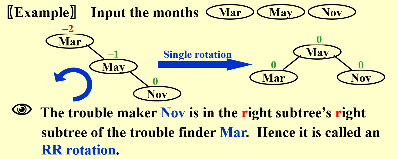
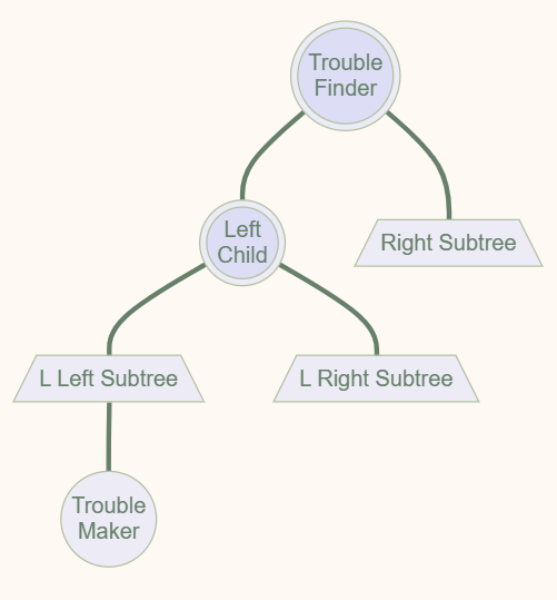
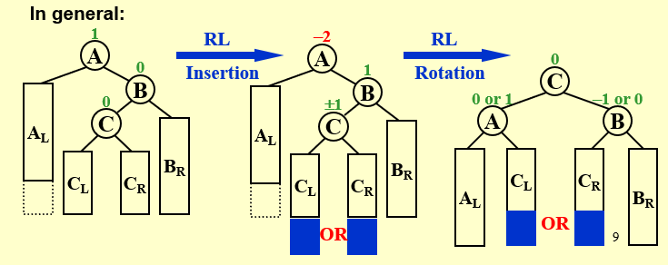
- Trouble maker 和 Trouble finder 之间的位置关系决定旋转的方式,一共分为 \(RR,RL,LR,LL\)
- Trouble Finder: 由于某个点的插入,导致 BF 不符合要求的点
- Related Trouble Finder’s Child
- Trouble Maker: 导致 Trouble Finder 出现的点
如下所示,在插入结点 5 后,此时根结点 8 的平衡因子 BF 值变为 2,不再满足 AVL Tree 的要求,而这一切都是 5 的插入导致的——于是我们称像这里的 8 一样,由于某个点的插入,其「平衡因子」不再符合要求的点,为 Trouble Finder;而像这里的 5 一样,导致 Trouble Finder 出现的点,被称之为 Trouble Maker。
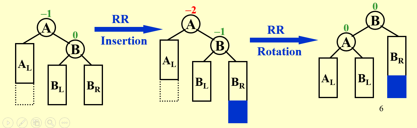
A结点不一定是根结点,当发现 RR 关系时,可以通过 局部的旋转 使树变得平衡
LL Single Rotation 的换根视角
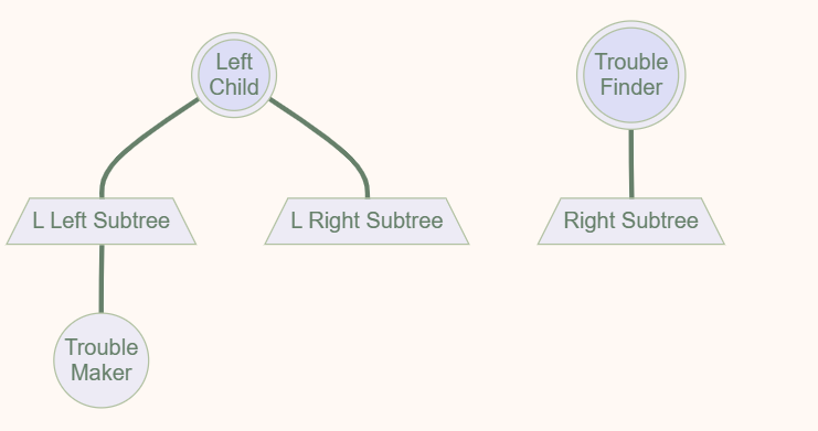
原先的根结点身处左子树的高台上,\(BF(root) = h_L - h_R = 2\), 所以要将根结点从台子上拉下来,此时顺理成章,左子树的根结点成为整棵树的根结点。
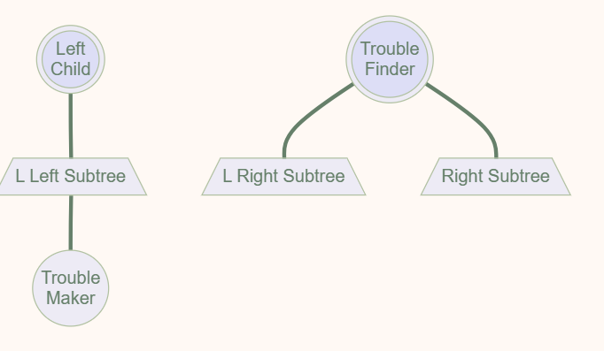
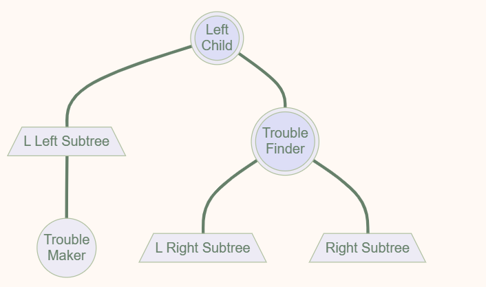
为了得到二分搜索树,需要将 Trouble Finder 与 左子树的根结点相连接,此时多出的 L Right Subtree 需要连接到 Trouble Finder。

以 B 为支点,先进行 C 的左旋,\(C_L\) 由于比 B 大,所以成为 B 的右子树;再进行 A 的右旋,A 比 C 大,成为 C 的右子树
为什么是最下面的点成为根结点呢?因为ABC三个点,能满足根结点的只有C,B < C < A
用语言概括就是,找到关键的那三个点,然后把最下面的顶到上面去,剩下两个作为左右孩子树,原先的那个点的左右孩子树则对应地,左孩子树接到左边空缺的右孩子树上,右孩子树接到右边空缺的左孩子树上。
如果一个Trouble maker插入后,产生了多个Trouble Finder,该如何处理?选择距离 Trouble maker 最近的 Trouble Finder 进行处理,最底层发生改变,连带效应引发上方的 Trouble Finder 的 BF 的绝对值都会减小。
int Height(AVLTree T)
{
    if(T) return T->height;
    // 空树 T == NULL
    else return -1;
}
void ChangeHeight(AVLTree T)
{
    if (T)
    {
        ChangeHeight(T->left);
        ChangeHeight(T->right);
        T->height = max(Height(T->left), Height(T->right)) + 1;
    }
}
int max(int a, int b)
{
    return a > b ? a : b;
}
AVLTree SingleRotateWithLeft(AVLTree T)
{
    AVLTree Newroot = (AVLTree)malloc(sizeof(TreeNode));
    Newroot = T->left;
    T->left = Newroot->right;
    Newroot->right = T;
    T->height = max(Height(T->left), Height(T->right)) + 1;
    Newroot->height = max(Height(Newroot->left), T->height) + 1;
    return Newroot;
}

AVLTree SingleRotateWithLeft(AVLTree T)
{
    AVLTree Newroot = (AVLTree)malloc(sizeof(TreeNode));
    // 旋转后的新根结点
    Newroot = T->left;
    // 旋转后结点关系的变化
    T->left = Newroot->right;
    Newroot->right = T;
    ChangeHeight(T);
    // T->height = max(Height(T->left), Height(T->right)) + 1;
    // Newroot->height = max(Height(Newroot->left), T->height) + 1;
    return Newroot;
}

AVLTree SingleRotateWithRight(AVLTree T)
{
    AVLTree Newroot = (AVLTree)malloc(sizeof(TreeNode));
    // 旋转后的新根结点
    Newroot = T->right;
    // 旋转后结点关系的变化
    T->right = Newroot->left;
    Newroot->left = T;
    // 旋转后更新树的高度
    ChangeHeight(T);
    // T->height = max(Height(T->left), Height(T->right)) + 1;
    // Newroot->height = max(Height(Newroot->right), T->height) + 1;
    return Newroot;
}
AVLTree DoubleRotateWithRight(AVLTree T)
{
    // RL
    // k3
    //      k2
    //  k1
    AVLTree newroot = (AVLTree)malloc(sizeof(TreeNode));
    T->right = SingleRotateWithLeft(T->right);
    // 此时 k3-k1-k2
    newroot = SingleRotateWithRight(T);
    return newroot;
}
// 定义AVL Tree的插入函数
AVLTree Insert(AVLTree T, int value)
{
    if(T == NULL)
    {
        T = (AVLTree)malloc(sizeof(TreeNode));
        T->data = value;
        T->height = 0;
        T->left = NULL;
        T->right = NULL;
    }
    else
    {
        if(value < T->data)
        {
            T->left = Insert(T->left, value);
            // 以上为二分搜索树的插入操作
            // 后续进行AVL Tree的平衡操作
            if(Height(T->left) - Height(T->right) == 2)
            {
                if(value < T->left->data)
                {
                    // LL
                    T = SingleRotateWithLeft(T);
                }
                else
                {
                    // LR
                    T = DoubleRotateWithLeft(T);
                }
            }
        }
        else if(value > T->data)
        {
            T->right = Insert(T->right, value);
            if(Height(T->right) - Height(T->left) == 2)
            {
                if(value > T->right->data)
                {
                    // RR
                    T = SingleRotateWithRight(T);
                }
                else
                {
                    // RL
                    T = DoubleRotateWithRight(T);
                }
            }
        }
        // 更新树的高度
        // T的高度等于左右子树中较高的高度加1
        T->height = max(Height(T->left), Height(T->right)) + 1;
    }
    return T;
}
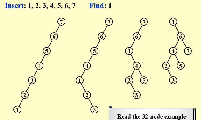
提问1: 在插入的时候是否有可能使多个结点的平衡性质被打破?
在 complete binary tree 的基础上,连续在左子树插入两个点,一条线上 \(O(log \ n)\) 个结点平衡性质被破坏
提问2: 如果是的话,一次旋转操作是否能使所有平衡收到破环的结点恢复正常?
\(LL,LR,RL,RR\) 旋转都会是插入的结点深度减少 1,所以路径上所有平衡被打破的结点都能恢复
定理2: AVL 树的搜索插入删除操作的时间复杂度都为O(log N)
对于搜索,典型的二叉搜索树,没有疑问。对于插入,最多两次旋转加上一次搜索。
对于删除操作,最多进行 \(O(log N)\) 次的旋转,而 每次旋转都是常数级别 的,时间复杂度仍为 \(O(log N)\)
AVLTree Delete(AVLTree T, int value)
{
    // 树为空,直接返回NULL
    if (T == NULL)
    {
        return NULL;
    }
    // 待删除的结点在T的左子树上
    if (value < T->data)
    {
        T->left = Delete(T->left, value);
        //删除结点后,如果AVL Tree失去平衡,则进行相应的调节
        if(Height(T->right) - Height(T->left) == 2)
        {
            AVLTree temp = T->right;
            if(Height(temp->left) > Height(temp->right))
            {
                T = DoubleRotateWithRight(T);
            }
            else
            {
                T = SingleRotateWithRight(T);
            }
        }
    }
    // 待删除的结点在T的右子树上
    else if (value > T->data)
    {
        T->right = Delete(T->right, value);
        if(Height(T->left) - Height(T->right) == 2)
        {
            AVLTree temp = T->left;
            if(Height(temp->right) > Height(temp->left))
            {
                T = DoubleRotateWithLeft(T);
            }
            else
            {
                T = SingleRotateWithLeft(T);
            }
        }
    }
    else
    {
        // 待删除的点在根结点
        if(T->left == NULL && T->right == NULL)
        {
            free(T);
            return NULL;
        }
        else if(T->right == NULL && T->left)
        {
            AVLTree temp = T;
            T = T->left;
            free(temp);
        }
        else if(T->left == NULL && T->right)
        {
            AVLTree temp = T;
            T = T->right;
            free(temp);
        }
        // 左右子树均非空,根据两棵树的height选择替换的结点
        else
        {
            if(Height(T->left) >= Height(T->right))
            {
                // 选择左子树中的最大值替换根结点
                AVLTree temp = T->left;
                while(temp->right)
                {
                    temp = temp->right;
                }
                int max = temp->data;
                T->data = max;
                T->left = Delete(T->left, max);
            }
            else
            {
                // 选择右子树中的最小值替换根结点
                AVLTree temp = T->right;
                while(temp->left)
                {
                    temp = temp->left;
                }
                int min = temp->data;
                T->data = min;
                T->right = Delete(T->right, min);
            }
        }
    }
    ChangeHeight(T);
    T->height = max(Height(T->left), Height(T->right)) + 1;
    return T;
}
1.2 Splay Tree
Splay Tree 的目标: 具体来说就是对于 \(M\) 次任意操作,其时间复杂度都为 \(O(MlogN)\),均摊下来这 \(M\) 个操作每一个都需要 \(O(logN)\)。
Splay 的核心思想就是,每当我们 访问一个结点(比如 查询 某个点、插入 某个点,甚至是 删除 某个点),我们就 通过一系列操作将目标点转移到根部,形象上理解就是不断旋转整个树的构造,知道把点转到根部。
-
搜索:使用普通二叉搜索树的方法找到结点,然后通过 splay 操作经过一系列旋转将搜索的结点移动到根结点的位置;
-
插入:使用普通二叉搜索树的方法找到要插入的位置进行插入,然后把刚刚插入的结点通过 splay 操作经过一系列旋转移动到根结点的位置;
-
删除:使用普通二叉搜索树的方法找到要删除的结点,然后通过 splay 操作经过一系列旋转将要删除的结点移动到根结点的位置,然后删除根结点(现在根结点就是要删除的点),然后和普通二叉搜索树的删除一样进行合理的 merge 即可。
先移到根结点,在进行删除
假如第一次访问,时间复杂度是 O(N), 那么第二次访问就是 O(1),因为此时该点已经位于根结点。
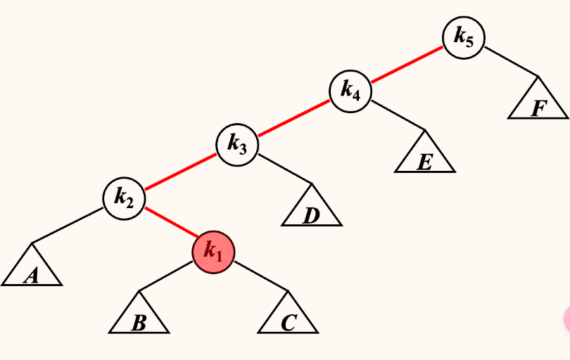
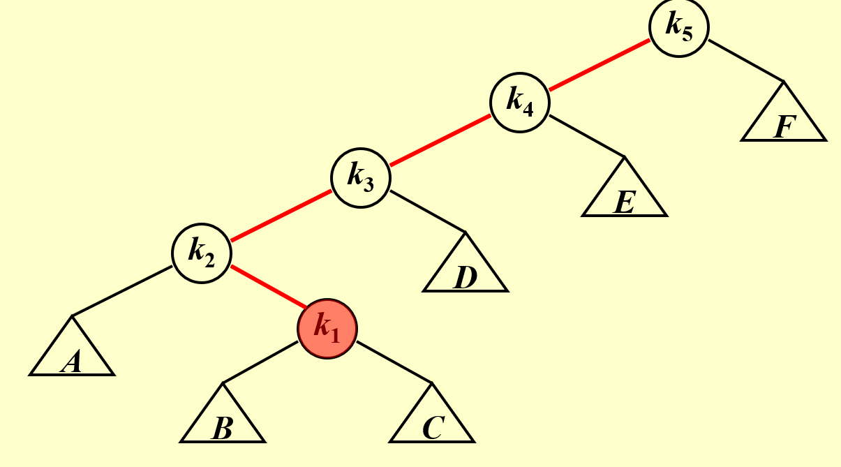
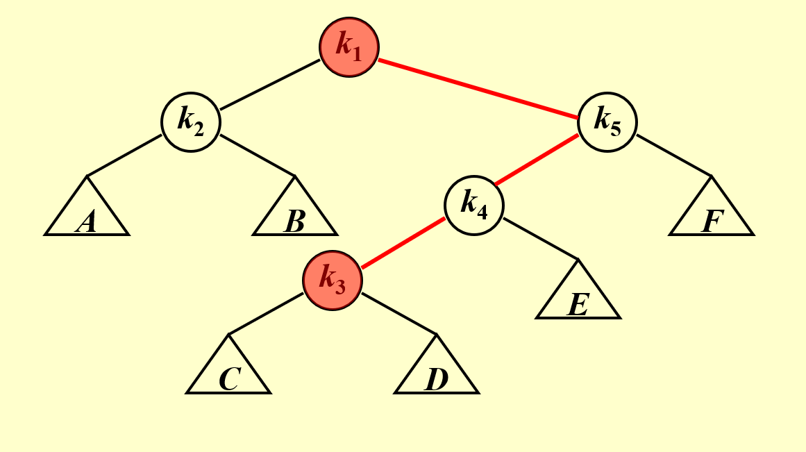
如图所示,此时 \(k1, k2, k3\) 对应 LR 的旋转关系,并且 \(k3\) 是最近的 Trouble Finder。
利用换根思想,以 \(k1\) 为根结点
要使根结点为 \(k1\) , 则将对 \(k4,k5\) 进行 两次 LL rotation。
第一次以 \(k4\) 为支点,对 \(k1,k4,k5\) 进行操作,此时得到 \(k4\) 为根结点,\(k5\) 成为 \(k4\) 的右子树,
第二次以 \(k1\) 为支点,对 \(k2,k1,k4进行操作\),\(k4\) 成为 \(k1\) 的右结点
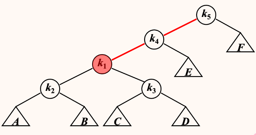
如何将上图所示,假如按照优先操作最近的 Trouble Finder 转化为 AVL Tree
LR rotation,\(k1\) 成为 \(k2,k3\) 的根结点
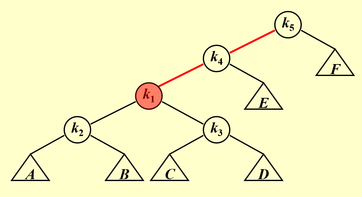
此时 \(k4\) 是最近的 Trouble Finder, 按照 LL rotatio 得到下图
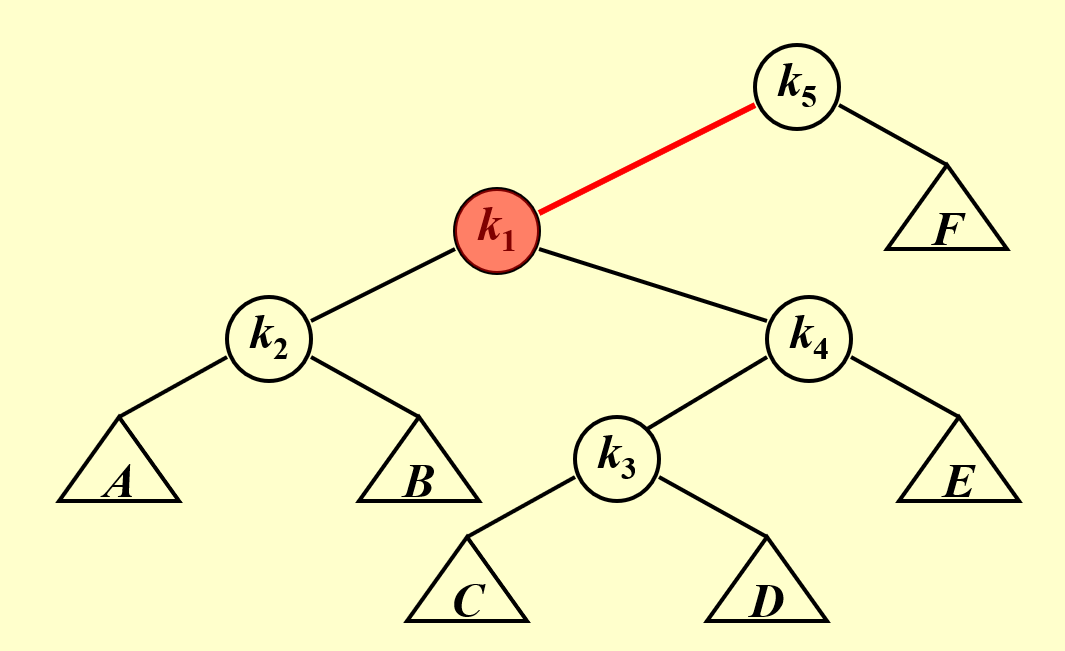
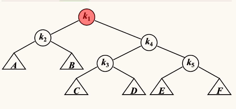
剩余 \(k5\) 是 Trouble Finder, 再进行一次 LL rotation
搜索 k1 的时间复杂度降低,但是搜索 k3 的时间复杂度增大,牺牲了某些点
此时你会发现,两次LL rotation 作用的顺序不一样,得到的结果可能是AVL Tree,也有可能不是。且与所得结论矛盾
以下引入,处理Splay Tree 的 处理方法
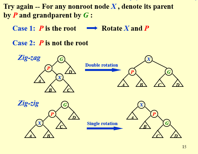
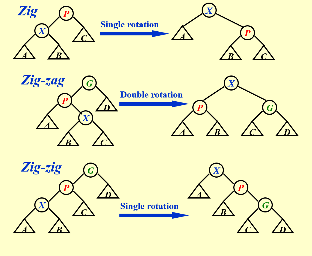
对于任意一个结点 X,我们记其父结点为 P(Parent),其父结点的父结点为 G(Grandparent)。
当我们访问到某个点 X 时:
-
如果 P 是根结点,则直接进行一次
[Single Rotation],将 X 转到根结点; -
如果 P 不是根结点
-
当情况为 LR / RL 时,进行一次
[LR Rotation / RL Rotation],我们称之为 zig-zag;不在一条直线上 -
当情况为 LL / RR 时,进行两次
[Single Rotation],使得 X、P、G 的顺序逆转,像跷跷板一样,我们称之为 zig-zig;在一条直线上此时 LL/RR 执行的顺序有严格要求,远端优先
zig-zig 是与 naive 的方法不一样的地方!
特别注意 naive 的方法
先交换X 和P 的位置关系,然后交换 X 和 G 的位置关系,但是 zig-zig 的标准操作方式是,
先交换P 和G 的位置关系,再交换 X 和 P 的位置关系!这个区别就是它与 naive 方法的唯一区别,却能实现我们最终均摊的目标;
1.3.2 对点操作
Splay Tree 除了在完成所有操作以后都需要进行一次 Splay 操作,其他部分都和 BST 一样。
- Find X
根据 BST 的性质,可以在 \(O(log N)\) 的时间内找到 X,接下来需要通过旋转操作,将 X 不断旋转至根结点
- Remove X
根据二分搜索树的性质,可以在 \(O(log N)\) 的时间内找到 X,接下来需要通过旋转操作,将 X 不断旋转至根结点。后续删除Root结点,找到左子树的最大值或者右子树的最小值,再进一步调整
- FindMax
根据 BST 的性质,可以在 \(O(log N)\) 的时间里找到最大值,将它旋转到根部以后,可以发现 它没有右孩子树,直接删掉就行。
#include <stdio.h>
#include <stdlib.h>

// 定义二分搜索树结构体
typedef struct SplayNode *SplayTree;
struct SplayNode
{
    int data;
    SplayTree left;
    SplayTree right;
    SplayTree parent;
} SplayNode;

SplayTree Insert(SplayTree T, int value);
SplayTree Find(SplayTree T, int value);
void Parent(SplayTree T);

SplayTree Insert(SplayTree T, int value)
{
    if (T == NULL)
    {
        T = (SplayTree)malloc(sizeof(SplayNode));
        T->data = value;
        T->left = T->right = NULL;
    }
    else
    {
        if (value < T->data)
        {
            T->left = Insert(T->left, value);
        }
        else if (value > T->data)
        {
            T->right = Insert(T->right, value);
        }
    }
    return T;
}
// 递归遍历树,建立父子关系
void Parent(SplayTree T)
{
    if (T->left)
    {
        T->left->parent = T;
        Parent(T->left);
    }
    if (T->right)
    {
        T->right->parent = T;
        Parent(T->right);
    }
}

SplayTree Find(SplayTree T, int value)
{
    if (T == NULL)
    {
        return NULL;
    }
    else
    {
        if (value < T->data)
        {
            return Find(T->left, value);
        }
        else if (value > T->data)
        {
            return Find(T->right, value);
        }
        else
        {
            return T;
        }
    }
}
SplayTree SingleRotateWithLeft(SplayTree T)
{
    SplayTree newroot = T->left;
    if (T->parent)
    {
        SplayTree G = T->parent;
        T->left = newroot->right;
        newroot->right = T;
        T->parent = newroot;
        newroot->parent = G;
        if(G->left == T)
            G->left = newroot;
        else
            G->right = newroot;
    }
    else
    {
        T->left = newroot->right;
        newroot->right = T;
        T->parent = newroot;
        newroot->parent = NULL;
    }

    return newroot;
}
SplayTree SingleRotateWithRight(SplayTree T)
{
    SplayTree newroot = T->right;
    if (T->parent)
    {
        SplayTree G = T->parent;
        T->right = newroot->left;
        newroot->left = T;
        T->parent = newroot;
        newroot->parent = G;
        if(G->left == T)
            G->left = newroot;
        else
            G->right = newroot;
    }
    else
    {
        T->right = newroot->left;
        newroot->left = T;
        T->parent = newroot;
        newroot->parent = NULL;
    }
    return newroot;
}

SplayTree DoubleRotateWithLeft(SplayTree T)
{
    SplayTree P = T->left;
    SplayTree newroot = P->right;
    if(T->parent)
    {
        SplayTree G = T->parent;
        T->left = SingleRotateWithRight(T->left);
        newroot = SingleRotateWithLeft(T);
        newroot->parent = G;
    }
    else
    {
        T->left = SingleRotateWithRight(T->left);
        newroot = SingleRotateWithLeft(T);
        newroot->parent = NULL;
    }
    return newroot;

}
SplayTree DoubleRotateWithRight(SplayTree T)
{
    SplayTree newroot = T->right->left;
    if(T->parent)
    {
        SplayTree G = T->parent;
        T->right = SingleRotateWithLeft(T->right);
        newroot = SingleRotateWithRight(T);
        newroot->parent = G;
    }
    else
    {
        T->right = SingleRotateWithLeft(T->right);
        newroot = SingleRotateWithRight(T);
        newroot->parent = NULL;
    }
    return newroot;
}
SplayTree RotatetoRoot(SplayTree T, int value)
{
    SplayTree temp = (SplayTree)malloc(sizeof(SplayNode));
    temp = Find(T, value);
    while (temp->parent != NULL)
    {
        SplayTree G = temp->parent->parent;
        SplayTree P = temp->parent;
        // 如果temp的父结点是根结点
        if (temp->parent == T)
        {
            // 直接进行一次SingleRotate,将temp旋转到根结点
            if (temp->parent->left == temp)
            {
                temp = SingleRotateWithLeft(temp->parent);
            }
            else
            {
                temp = SingleRotateWithRight(temp->parent);
            }
        }
        // 如果temp的父结点不是根结点
        else
        {
            // 按照Zig-zig 或者 Zig-zag分类讨论
            // LL型 zig-zig
            if (G->left == P && P->left == temp)
            {
                P = SingleRotateWithLeft(G);
                temp = SingleRotateWithLeft(P);
            }
            // RR型 zig-zig
            else if (G->right == P && P->right == temp)
            {
                P = SingleRotateWithRight(G);
                temp = SingleRotateWithRight(P);
            }
            // LR型 zig-zag
            else if (G->left == P && P->right == temp)
            {
                temp = DoubleRotateWithLeft(G);
            }
            // RL型 zig-zag
            else if (G->right == P && P->left == temp)
            {
                temp = DoubleRotateWithRight(G);
            }
        }
    }
    return temp;
}

void Levelorder(SplayTree T)
{
    SplayTree queue[100];
    int front = 0, rear = 0;
    int currentLevelCount = 1, nextLevelCount = 0;
    if (T == NULL)
    {
        return;
    }
    queue[rear++] = T;
    while (front < rear)
    {
        SplayTree temp = queue[front++];
        printf("%d ", temp->data);
        currentLevelCount--;
        if (temp->left)
        {
            queue[rear++] = temp->left;
            nextLevelCount++;
        }
        if (temp->right)
        {
            queue[rear++] = temp->right;
            nextLevelCount++;
        }
        if (currentLevelCount == 0)
        {
            printf("\n");
            currentLevelCount = nextLevelCount;
            nextLevelCount = 0;
        }
    }
}
int main()
{
    SplayTree T = NULL;
    T = Insert(T, 10);
    T = Insert(T, 4);
    T = Insert(T, 11);
    T = Insert(T, 2);
    T = Insert(T, 6);
    T = Insert(T, 12);
    T = Insert(T, 1);
    T = Insert(T, 3);
    T = Insert(T, 5);
    T = Insert(T, 8);
    T = Insert(T, 7);
    T = Insert(T, 9);
    T = Insert(T, 13);
    Parent(T);
    T->parent = NULL;
    T = RotatetoRoot(T, 3);
    Levelorder(T);
    Parent(T);
    T->parent = NULL;
    T = RotatetoRoot(T, 9);
    Levelorder(T);
    Parent(T);
    T->parent = NULL;
    T = RotatetoRoot(T, 1);
    Levelorder(T);
    Parent(T);
    T->parent = NULL;
    T = RotatetoRoot(T, 5);

    Levelorder(T);
}
对于 Insert 操作
SplayTree RotatetoRoot(SplayTree T, int value)
{
    SplayTree temp = (SplayTree)malloc(sizeof(SplayNode));
    T = Insert(T, value);
    Parent(T);
    temp = Find(T, value);
    while (temp->parent != NULL)
    {
        SplayTree G = temp->parent->parent;
        SplayTree P = temp->parent;
        // 如果temp的父结点是根结点
        if (temp->parent == T)
        {
            // 直接进行一次SingleRotate,将temp旋转到根结点
            if (temp->parent->left == temp)
            {
                temp = SingleRotateWithLeft(temp->parent);
            }
            else
            {
                temp = SingleRotateWithRight(temp->parent);
            }
        }
        // 如果temp的父结点不是根结点
        else
        {
            // 按照Zig-zig 或者 Zig-zag分类讨论
            // LL型 zig-zig
            if (G->left == P && P->left == temp)
            {
                P = SingleRotateWithLeft(G);
                temp = SingleRotateWithLeft(P);
            }
            // RR型 zig-zig
            else if (G->right == P && P->right == temp)
            {
                P = SingleRotateWithRight(G);
                temp = SingleRotateWithRight(P);
            }
            // LR型 zig-zag
            else if (G->left == P && P->right == temp)
            {
                temp = DoubleRotateWithLeft(G);
            }
            // RL型 zig-zag
            else if (G->right == P && P->left == temp)
            {
                temp = DoubleRotateWithRight(G);
            }
        }
    }
    return temp;
}
只需在 RotateToRoot 函数中,先插入指定值 value,建立 parent 关系,再找到该 value,进行旋转到 root
删除:
使用普通二叉搜索树的方法找到要删除的结点,然后通过splay 操作经过一系列旋转将要删除的结点移动到根结点的位置,
然后删除根结点(现在根结点就是要删除的点),然后和普通二叉搜索树的删除一样进行合理的merge 即可。
(AVL树和Splay树的旋转代码区别在于:AVL树的旋转选取的是height更大的结点作为基准点,也就是高位的结点,因为插入一个点后,要确保高位以下的结点的height都得到更新,这样才能计算高位的平衡因子>=2.
但是在splay树中,我们都是先找到目标结点,显然它是在下方,我们需要根据它的parent和grandparent的位置,确定当前的旋转方式。所以旋转的代码是以下位的点作为基准点。此时略有问题,可忽略不看)
1.3 Amortized Analysis
Any M consecutive operations take at most O(M log N) time. -- Amortized time bound
它计算的是从初始状态开始,连续的 M 次任意操作 最多有 的代价。
需要注意的是,它不同于平均时间分析(所有可能的操作出现概率平均,也就是直接求平均)和概率算法的概率分析(平均话所有可能的随机选择,也就是加权求平均)不同,摊还分析和概率完全无关。
worse-case bound >= amortized bound >= average-case bound
针对上方的不等式,由于 amortized bound 限制了所有的 M 次操作,所以其上界就等于最差的情况发生 M 次。(由于 amortized bound 是连续的 M 次任意操作 最多有 的代价。)average bound 存在稀释,所以大于等于平均情况
对于上界等于最差的情况发生 M 次,忽略了有的序列是不可能出现的。例如在空树上用 \(O(N)\) 的时间进行删除。
摊还分析则是希望排除最差情况分析中不可能的情况。注意点:
摊还分析要求从空结构开始,。否则可以思考从一个已经有很多元素的栈里面一次性 Multipop 出所有元素,这一步操作的复杂度显然不再是 O(1 · 1) 的
1.3.1 aggregate analysis 聚合法
Show that for all n, a sequence of n operations takes worst-case time (\(T(n)\)\) in total. In the worst case, the average cost, or amortized cost, per operation is \(T(n)/n\)
// stack with multipop
void MultiPop(int k, Stack S)
{
    while(!IsEmpty(S) && k > 0)
    {
        Pop(S);
        k--;
    }
}
// T = min(sizeof(S), k)
Consider a sequence of n Push, Pop, and MultiPop operations on an initially empty stack.
均摊付出的最大代价是:\(n-1\) 次 \(push\),1 次 \(multipop\)
\(T(n) = (n-1)O(1) + O(n-1) = O(n)\)
\(T_{amortized} = O(n) / n = O(1)\)
1.3.2 accounting method 核算法
截长补短
记 \(credit = amortized \ cost \ \widehat c_i - actual \ cost \ c_i\)
对所有的 n 次操作而言,都有

目的是满足之前的不等式,保证摊还成本平均成本大 \(\sum_{i = 1}^n credit_i >=0\)
举个例子说明上述不等式
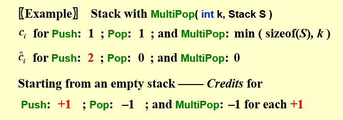
因为我们希望一次操作摊还成本为 O(1),所以我们希望这三种操作的成本都是 常数级别 的,这样只要使得 \(\sum_{i = 1}^n credit_i >=0\),那就直接证明了结论。但是我们知道,MultiPop 的代价比较大,把它调整为常数,对应的 \(\Delta < 0\),必然需要代价小的操作 \(\Delta > 0\),所以才有了例子中把 Push 操作代价调整为 2,然后我们可以 利用 size(S) ⩾ 0 这一约束证明 \(\sum_{i = 1}^n credit_i >=0\)
栈内有剩余,说明 multipop 没有发挥全力,导致实际成本小于均摊成本。
均摊成本的考量在于,使栈内没有剩余,意味着 push 一定 pop,这样 push 的成本变为 2,包含了 pop 和 multipop
1.3.3 potential method 势能法
上面的核算法相对形象,但要为每一个操作设计一个摊还代价 \(\widehat c_i = c_i + \Delta_i\) 并不像上述例子那么简单,况且需要保证 \(\sum_{i=1}^n \Delta_i >= 0\).对于比较复杂的结构,如 splaytree,就很难办.
定义一个势能函数,第 i 次操作 的摊还代价是 \(\widehat c_i = c_i + (\phi(D_i)-\phi(D_{i-1}))\)
\(D_i\) 是第 i 次操作之后的数据结构,\(\phi(D_i)\) 表示第 i 次操作之后的势能
每一步的摊还代价等于真实操作的代价加上势函数的变化
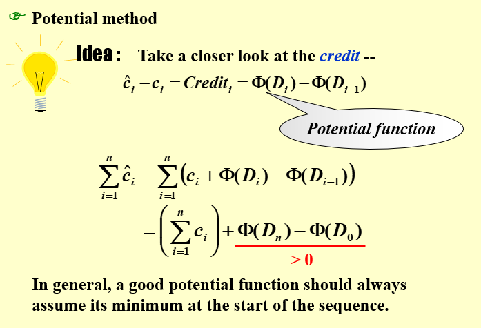
为了使得摊还成本是平均成本的上界,我们仍然需要满足 \(\sum_{i=1}^n \widehat c_i >= \sum_{i=1}^n c_i\), 因此只需要满足 \(\phi(D_n) >= \phi(D_0)\)
只需要调整设计,初始状态时$\phi(D_0)$最小,等于0,后续的每一步操作势能都不会小于0
如果 \(\sum_{i=1}^n c_i = O(log N)\),合理的势能函数选择应该满足 \(Φ(Dn) − Φ(D0)\) 也是 \(O(log n)\),否则会影响估算的精确度。
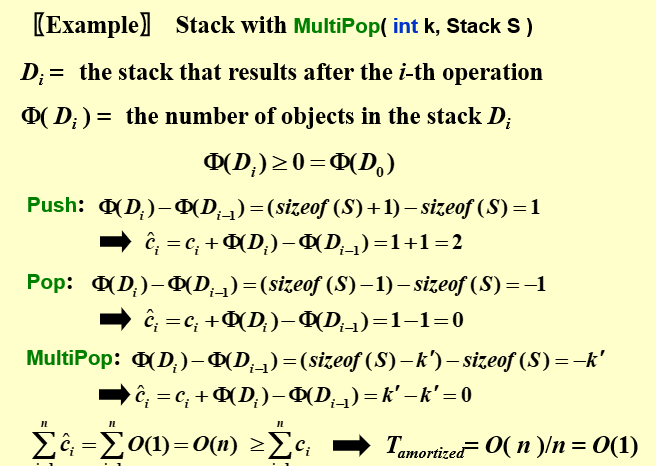
针对上述例子,定义势能函数为栈中存在的元素个数
1.3.4 Splay Tree 的 摊还分析
我们考虑一个跟结点高度相关的(或类似的)势能函数。
我们注意到在 Splay 操作中,几乎每个结点的高度都会改变,哪怕该结点为根结点的子树没有任何变化。如果我们直接使用结点高度作为势能函数,后续的数学计算与推导会变得非常复杂。
一个可用的势能函数是树中所有结点的 rank 之和:
\(S(i)\) 指的是子树 \(i\) 的结点数,包括结点 \(i\).
\(R(i)\) 表示结点 \(i\) 的 rank,\(R(i) = logS(i)\)
选取 rank 之和作为势能函数的好处是除了 X, P, G 三个结点外,其他结点在 splay 操作中 rank 保持不变,因而可以简化计算。
- Zig: 在整个操作中只有 X 和 P 的 rank 值有变化。
其中 \(R_2(X) -R_1(X) > 0 , R_2(P)-R_1(P) <= 0\)
所以 \(\widehat c_i <= 1 + R_2(X) - R_1(X) <= 1 + 3(R_2(X) - R_1(X))\)
- Zig-Zag: 两次旋转
引理: 若 \(a + b <= c\), 且 \(a ,b\) 均为正整数,则 \(log a+ log b <= 2logc -2\)
- Zig-zig:两次旋转 最后,给定一个伸展树上访问节点 X 的一系列 M 个 splay 操作(zig、zigzig、zigzag),其中最多只会有 1 个 zig。把他们都给加起来后,可得:
上面证明每一次操作的均摊成本都是 \(O(logN)\) 级别。考虑到上课有个例子对退化成链表的树的叶结点做 Splay 操作,复杂度为 \(O(n)\)。是否产生矛盾?
这并不矛盾,一个是 均摊成本,一个是 真实成本
我们应该证明M个连续操作的成本不大于$O(MlogN)$
令 \(T_0\) 为操作前的 splay Tree,为空树。\(T_i\) 为第 \(i\) 次操作后的伸展树(\(1 <= i <= M\)), \(c_i\) 为第 \(i\) 次操作的实际成本
定理:Splay 树的搜索、插入和删除操作的摊还复杂度均为 \(O(log n)\)。
1.4 习题集
-
If the depth of an AVL tree is 6 (the depth of an empty tree is defined to be -1), then the minimum possible number of nodes in this tree is:
-
A. 13
-
B. 17
-
C. 20
-
D. 33
前面的递推关系式 \(N_h = N_{h-1} + N_{h-2} + 1, N_0 = 1, N_1 = 2\)
那么 \(N_2 = 4, N_3 = 7, N_4 = 12, N_5= 20, N_6= 33\)
-
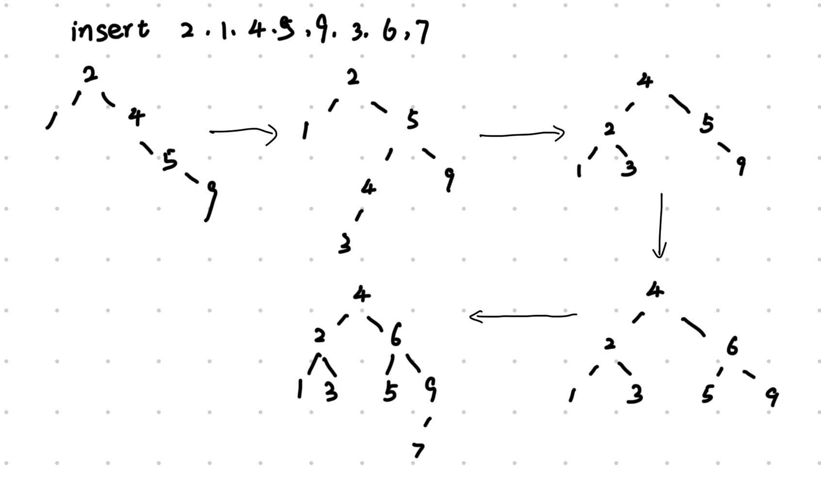
Insert 2, 1, 4, 5, 9, 3, 6, 7 into an initially empty AVL tree. Which one of the following statements is FALSE?
-
A. 4 is the root
-
B. 3 and 7 are siblings -
C. 2 and 6 are siblings
-
D. 9 is the parent of 7
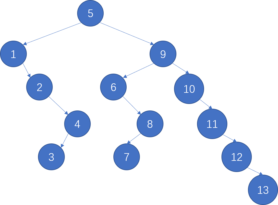
- For the result of accessing the keys 3, 9, 1, 5 in order in the splay tree in the following figure, which one of the following statements is FALSE?
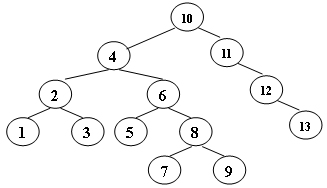
-
A. 5 is the root
-
B. 1 and 9 are siblings
-
C. 6 and 10 are siblings
-
D. 3 is the parent of 4
5
1 9
2 6 10
4 8 11
3 7 12
13
-
When doing amortized analysis, which one of the following statements is FALSE?
-
A. Aggregate analysis(聚合法) shows that for all \(n\), a sequence of \(n\) operations takes worst-case time \(T(n)\) in total. Then the amortized cost per operation is therefore \(T(n)/n\)
-
B.
For potential method(势能法), a good potential function should always assume its **maximum** at the start of the sequence势能法,要求初始时刻的势能最小 -
C. For accounting method(核算法), when an operation's amortized cost exceeds its actual cost, we save the difference as credit to pay for later operations whose amortized cost is less than their actual cost
-
D. The difference between aggregate analysis and accounting method is that the later one assumes that the amortized costs of the operations may differ from each other
聚合法是求平均,假设的是 amortized cost 是相等的。account 法假设的是 amortized cost 是不相等的每次操作。当操作的摊余成本超过其实际成本时,我们会将差额存为 credit,以支付摊余成本低于其实际成本的后续操作
-
Consider the following buffer management problem. Initially the buffer size (the number of blocks) is one. Each block can accommodate exactly one item. As soon as a new item arrives, check if there is an available block. If yes, put the item into the block, induced a cost of one. Otherwise, the buffer size is doubled, and then the item is able to put into. Moreover, the old items have to be moved into the new buffer so it costs \(k+1\) to make this insertion, where \(k\) is the number of old items. Clearly, if there are \(N\) items, the worst-case cost for one insertion can be \(\Omega (N)\). To show that the average cost is \(O(1)\), let us turn to the amortized analysis. To simplify the problem, assume that the buffer is full after all the \(N\) items are placed. Which of the following potential functions works?
A. The number of items currently in the buffer
B. The number of blocks currently in the buffer
C. The number of available blocks currently in the buffer
D.
The opposite number of available blocks in the buffer