12. Local Search¶

约 4823 个字 27 行代码预计阅读时间 24 分钟

Local

local optimum is a best solution in a neighborhood

Search

start with a feasible solution and search a better one within the neighborhood
a local optimum is achieved if no improvement is possible

① 得到一个初始的可行解

② 每一轮循环中，从这个可行解的邻域中，选择邻域最优解作为新的可行解。

③ 假如这个可行解的邻域中没有任何一个解优于这个可行解，退出循环，返回结果。

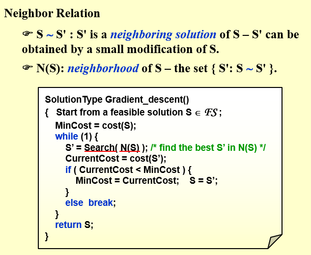
梯度下降算法，局部搜索找到点使得，current cost < mincost

12.1 The Vertex Cover Problem¶

有附带条件，size <= K , 该问题是一个NP-complete问题

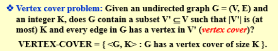
顶点覆盖问题(vertex cover problem)指给定一个无向图$G=(V,E)$，找到一个最小的顶点集$S\subseteq V$，使得每条边$(u,v)$都至少有一个端点在$S$中（即$u\in S \lor v\in S$）。

该问题是一个NP-Hard问题。暂时无法找到一个多项式时间的算法来解决这个问题

这个问题的可行解为$S = V$，即完全覆盖，其目标函数为$cost(S) = |S|$。即，我们尝试使用 local search 来降低$|S|$。

Search: Start from S = V; delete a node and check if S' is a vertex cover with a smaller cost.

给出几种案例以及可视化，说明局部搜索容易失效。

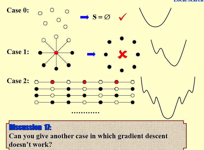
case 0：没有边，显然顶点覆盖子集为空
case 1：最优顶点覆盖子集为中心点。假如我们从S=V入手，假设先去掉中心点，剩下的8个点仍然是顶点覆盖子集，但是无法再删除（局部最优解）。如果先删除周围的点，才有可能得到全局最优解。说明局部搜索存在失效的可能
case 2：存在多个局部最优解，但是不是全局最优解

当成本函数是非凸函数且具有多个局部最小值时，梯度下降可能无法有效地工作。在这种情况下，梯度下降可能会陷入局部最小值，而不是收敛到全局最小值。这是因为梯度下降根据成本函数的局部梯度更新参数，如果它恰好从一个初始点开始，该点接近一个局部最小值但远离全局最小值，那么它可能会收敛到该局部最小值。

为了缓解这个问题，常用的方法是使用随机梯度下降（SGD）或其变体，如Adam、RMSprop或AdaGrad，这些方法引入了随机性或自适应学习率，以帮助跳出局部最小值并找到更好的解决方案。

12.2 metropolis algorithm¶

梅特罗波利斯算法(the Metropolis algorithm)的过程：

SolutionType Metropolis()
{
    Define constants k and T;
    Start from a feasible solution S \in FS;
    MinCost = cost(S);
    while (1)
    {
        S’ = Randomly chosen from N(S);
        CurrentCost = cost(S’);
        if (CurrentCost < MinCost)
        {
            MinCost = CurrentCost;
            S = S’;
        }
        else
        {
            With a probability e ^ { -\Delta cost / (kT) }, let S = S’;
            else break;
        }
    }
    return S;
}

在局部搜索算法中加⼊⼀个概率p，如果当邻点的值优于当前点时我们接受它；当邻点的值劣于当前点时我们也有p的概率仍然接受它。这就带来了在反复迭代中跳出局部最优解的机会。
概率p的大小受到当前点的值的影响，当前点值越靠近期望的⽅向（即温度越低），p的值越小。这使当前点落⼊较优的解空间时更不容易跳出，即更稳定的能获得优值。

注：当（温度）T很高时，上坡的概率几乎为1，容易引起底部震荡；当T接近0时，上坡概率几乎为0，接近原始的梯度下降法。

Metropolis算法当然也存在需要优化的地方（对于简单问题，存在较大概率选择到一个比当前解差的情况，但是又有一定的概率接受这个解，这样就会偏离最优解，甚至陷入在几个解之间来回跳跃但就是找不到最优解的境地）。

观察metropolis算法的一个重要参数之后，发现高温有利于跳出局部最优解，温度较低时，进入最优解后不易跳出。因此我们希望在开始的时候温度很高，然后逐渐降低温度，这样在开始时我们能够跳出局部最优解，在逐渐降温后停留在最优解。这实际上就是模拟退火的思想

模拟退火(simulated annealing)

Cooling schedule: T = { T1 , T2 , … }

12.3 Hopfield Neural Networks¶

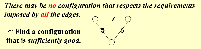
Graph$G = (V, E)$with integer edge weights w (positive or negative).

If$w_e$< 0, where$e = (u, v)$, then u and v want to have the same state;

if$w_e > 0$then u and v want different states.

The absolute value$|w_e|$indicates the strength of this requirement.

绝对值$|w_e|$表示此要求的强度。

Hopfield 神经网络可以抽象为一个无向图$G = (V,E)$，其中$V$是神经元的集合，$E$是神经元之间的连接关系，并且每条边$e$都有一个权重$w_e$，这可能是正数或负数；
对网络中每个神经元（即图的顶点）的状态的一个赋值，赋值可能为$1$或$-1$，我们记顶点$u$的状态为$s_u$；
如果对于边$e = (u, v)$有$w_e > 0$，则我们希望$u$和$v$具有相反的状态；如果$w_e < 0$，则我们希望$u$和$v$具有相同的状态；综合而言，我们希望$w_es_us_v < 0$
我们将满足上述条件的边$e$称为“好的（$good$）”，否则称为“坏的（$bad$）”；
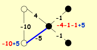
我们称一个点u 是“满意的（$satisfied$）”，当且仅当$u$所在的边中，好边的权重绝对值之和大于等于坏边的权重绝对值之和 $$ \underset{v:e=(u,v)\in E}{\sum}w_es_us_v \leq 0 $$
我们称一个构型是“稳定的（stable）”，当且仅当所有的点都是满意的

Output: A configuration S of the network – an assignment of the state$s_u$to each node u

〖Definition〗 In a configuration S, edge$e = (u, v)$is good if$w_e s_u s_v < 0$($w_e < 0$iff$s_u = s_v$); otherwise, it is bad.

〖Definition〗 In a configuration S, a node u is satisfied if the weight of incident good edges$\geq$ weight of incident bad edges. $$ \sum_{v:e=(u,v)\in E} w_es_us_v \leq 0 $$ 由于不一定能找到完美的configuration，所以退而求其次，要求好边的权重大于外边的权重

〖Definition〗A configuration is stable if all nodes are satisfied.

Does a Hopfield network always have a stable configuration, and if so, how can we find one?

如果一个结点不满足，那么我就把这个结点的state取反（因为仅有满足和不满足），取反之后与该点相连的边，好边变坏边，坏边变好边

关键问题是：Will it always terminate？是否总会停止

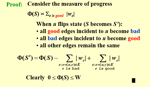
每一次取反之后，该点的好边权重至少+1，但是总权重是有限的，所以一定会停止

Claim: The state-flipping algorithm terminates at a stable configuration after at most$W = _e|w_e|$iterations.
Proof:
Problem: To maximize$\Phi$

$S - S'$:$S'$can be obtained from S by flipping a single state

Claim: Any local maximum in the state-flipping algorithm to maximize$\Phi$is a stable configuration.

他是否是多项式时间算法？

Still an open question: to find an algorithm that constructs stable states in time polynomial in$n$and$logW$(rather than n and W), or in a number of primitive arithmetic operations that is polynomial in n alone, independent of the value of W.

仍然是一个悬而未决的问题：找到一种算法，该算法在 n 和 logW（而不是 n 和 W）中构造时间多项式中的稳定状态，或者在一些原始算术运算中构造稳定状态，该运算仅在 n 中是多项式的，与 W 的值无关。

12.4 The Maximum Cut Problem¶

Maximum Cut problem: Given an undirected graph$G = (V, E)$with positive integer edge weights we, find a node partition$(A, B)$such that the total weight of edges crossing the cut is maximized. $$ w(A,B) = \sum_{u\in A, v\in B} w_{uv} $$ 应用：n项活动，M项人。每个人都想参加其中两项活动。将每项活动安排在上午或下午，以最大限度地增加可以享受这两项活动的人数。

problem： To maximize $\Phi(S) = \sum_{e \ is \ good}|w_e|$
Feasible solution set FS : any partition (A, B)
S - S': S' can be obtained from S by moving one node from A to B, or one from B to A.

最大割问题和Hopfield神经网络问题存在着关联。对于任意解（A，B），将A中的点的状态赋值为-1，B中的点的状态赋值为1.此时组内的边变为坏边（$w_es_us_v >0$）,组间的边变为好边，问题转化为最大化好边的总权重之和$\Phi(S)$.

移动一点从组A到组B，与该点相连的变，组间的变组内，组内的变组间

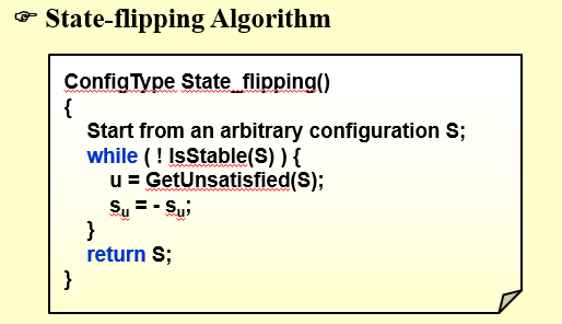
ConfigType State_flipping()
{
    Start from an arbitrary configuration S;
    while ( ! IsStable(S) ) {
        u = GetUnsatisfied(S);
        su = - su;
    }
    return S;
}

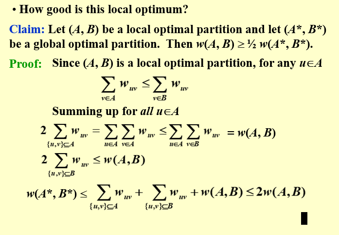
即图G中所有边的权重之和为$W = \underset{(u,v)\in E}{\sum}w_{uv}$,因为（A，B）是一个局部最优解，即把u放到B会使割边的权重和降低，也就是说对于任意一个在A中的点u，满足组间权重之和大于组内权重之和即$\underset{v\in A}{\sum}w_{uv} \leq \underset{v \in B}{\sum}w_{uv}$

这是因为原先点u的好边权重之和大于坏边权重之和，一旦从A移动到B之后，原先的好边变为坏边，坏边变为好边，导致好边的权重降低

对所有的$u \in A$都有这样的不等式，对所有的不等式求和得到 $$ \underset{u \in A}{\sum} \underset{v \in A}{\sum}w_{uv} \leq \underset{u \in A}{\sum} \underset{v \in B}{\sum}w_{uv} $$ 显然左边是2倍的A中所有边的权重之和，因为每一条边计算了两次，右边使所有的割边的权重之和 $$ 2\underset{(u,v) \in A}{\sum} w_{u,v} = \underset{u \in A}{\sum} \underset{v \in A}{\sum}w_{uv} \leq \underset{u \in A}{\sum} \underset{v \in B} {\sum}w_{uv} = w(A,B) \ 对(u,v) \in B 同理 $$ 组间权重要大于组内权重，组间权重在总权重中至少要占1/2

总权重$W = \underset{(u,v) \in A}{\sum} w_{u,v} + \underset{(u,v) \in B}{\sum} w_{u,v} + w(A, B)$, 由于最大割的权重之和不会超过全体边的权重和W，所以$w(A^*,B^*) \leq W = \underset{(u,v) \in A}{\sum} w_{u,v} + \underset{(u,v) \in B}{\sum} w_{u,v} + w(A, B) \leq 2w(A,B)$

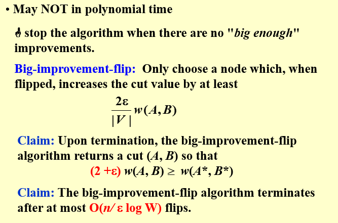
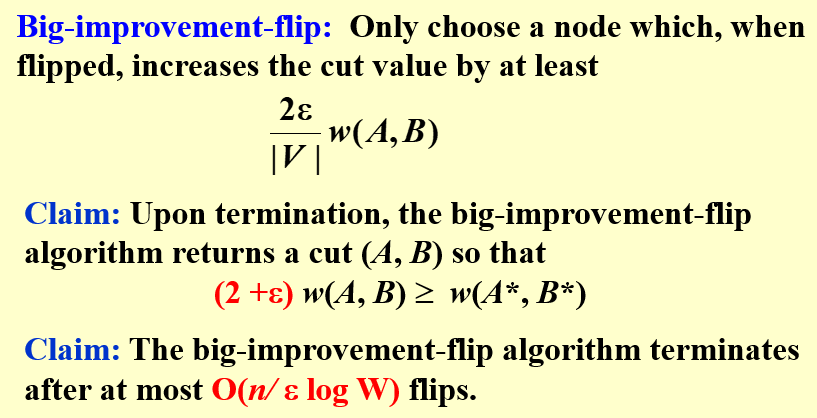
设置一个阈值，要求每一次权重的增加需要大于阈值

如果添加阈值，$\dfrac{2\epsilon }{|V|} w(A,B)$,那么最终得到的结果满足$w(A^*,B^*) \leq (2 + \epsilon)w(A,B)$

最终翻转$O(n/\epsilon logW)$次

如果不添加阈值，最终得到的结果满足$w(A^*,B^*) \leq 2w(A,B)$

12.5 旅行商问题¶

定义：给定一个无向完全图$G = (V,E)$,每条边$(u,v) \in E$有一个权重$w(u,v)$,我们希望找到一个最短回路，使得每一个顶点都被恰好访问一次，并且所付出的代价最少。

这是一个NP-Hard问题，暂时找不到一个多项式时间算法来解决这个问题

12.5.1 动态规划¶

假设我们给所有顶点编号为1，2，3，4....，n，然后我们的目标时找一条最短的经过每一点恰好从1回到1（起始点任意，回路等价）的哈密顿回路。那么这个路径的最后一跳应当是从某个点$j != 1$,那么我们的问题转化为找最优的点$j$完成最后一跳。 $$ 最优路线的成本 = min_{j = 2,3,...n}访问每个顶点的无环1\rightarrow j路径的最低成本 + c_{j1} $$ 这里我们就要用最短路问题自带的最优子结构来设计动态规划算法了（我们在Bellman-Ford 和Floyd-Warshall 算法中已经实践过）：即最短路径的某一段也一定是对应的起点终点的最短路径。因此如果我们要求从$1$到$j$的最短路径，我们可以考虑最后一跳的选取，假设最短路径最后一跳是从$k$到$j$，那么我们可以将问题分解为从$1$到$k$的最短路径加上从k 到j 的成本.

当然我们并不能直接知道哪个$k$最好，所以还需要遍历所有的$k$，这样就决定了最后一跳。然后我们递归解决倒数第二跳，以此类推。我们不难发现，这样的动态规划算法的子问题可以表达为$C_{S,j}$,表示从1到$j \in S$经过S中所有点恰好一次的最短路径。 $$ C_{S,j} = \underset{k \in S, k != 1,j}{min} C_{S-{j},k}+c_{k,j} $$ 根据递推式的特点，我们只要按照S的大小从小到大依次填表，就能保证解每一个问题的时候，需要的子问题的答案都已知。

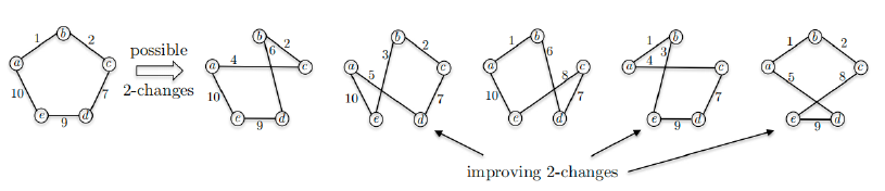
12.5.2 局部搜索¶

定义邻居关系：对于两条长度为n的不同的哈密顿回路，它们之间能共享的最大边数为n-2，因此我们定义两条哈密顿回路S和S‘之间的邻居关系为：S和S’之间的边有两条不一样

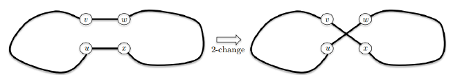
接下来就可以在2-近似的解的基础上做2-变换进一步改进解（即检查改变之后受到影响的边的长度是否减小）

12.6 习题集¶

Q1-1. For the graph given in the following figure, if we start from deleting the black vertex, then local search can always find the minimum vertex cover. (T/F)

T

一个点可以删除的条件是：这条边的另一个点没有被删除。如果可以删除，则任意删除一个。如果不能删除，则算法结束。剩下的点越少越好。

如果删除黑点，那么不能删除右边的点，也不能删除下面的点，只能删除最下面两个。因此确实达到了最优解。

Q1-2. We are given a set of sites$S=\{s_{1}, s_{2}, \cdots, s_{n}\}$in the plane, and we want to choose a set of$k$centers$C=\{c_{1}, c_{2}, \cdots, c_{k}\}$so that the maximum distance from a site to the nearest center is minimized. Here$c_{i}$can be an arbitrary point in the plane.

A local search algorithm arbitrarily choose$k$points in the plane to be the centers, then
- (1) divide$S$into$k$sets, where$S_{i}$is the set of all sites for which$c_{i}$is the nearest center; and
- (2) for each$S_{i}$, compute the central position as a new center for all the sites in$S_{i}$.
If steps (1) and (2) cause the covering radius to strictly decrease, we perform another iteration, otherwise the algorithm stops.

When the above local search algorithm terminates, the covering radius of its solution is at most 2 times the optimal covering radius. (T/F)

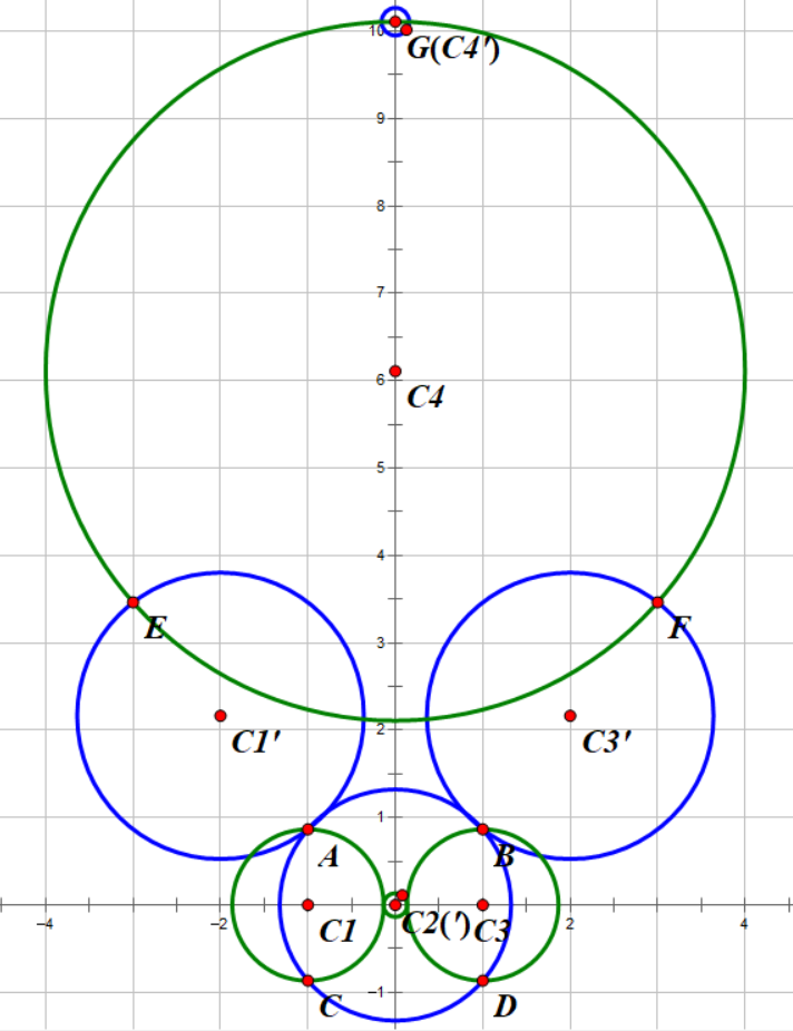
F原因在于K center近似比不能低于2.否则P=NP

给出反例如下图所示。其中有

$$ \begin{gathered} A(-1, \frac{\sqrt{3}}{2}),\quad B(1, \frac{\sqrt{3}}{2}),\quad C(-1, -\frac{\sqrt{3}}{2}),\quad D(1, -\frac{\sqrt{3}}{2}) \end{gathered} $$

$$ \begin{gathered} E(-3, 2\sqrt{3}),\quad F(3, 2\sqrt{3}),\quad G(0, 2\sqrt{3}+\sqrt{7}),\quad H(0,0.000001),\quad I(0,-0.000001) \end{gathered} $$

都是需要被覆盖的点。

$$ c_1(-1, 0),\quad c_2(0, 0),\quad c_3(1, 0),\quad c_4(0, 2\sqrt{3}+\sqrt{7}),\quad $$

$c_1$,$c_3$半径为$\frac{\sqrt{3}}{2}$,$c_2$半径为$0.0001$,$c_4$半径为$4$。这样得到的解就是 Local Search 的一个可能解，覆盖半径为$4$。

然而，如果取

$$ c_1'(-2, \frac{5\sqrt{3}}{4}),\quad c_2'(0, 0),\quad c_3'(2, \frac{5\sqrt{3}}{4}),\quad c_4'(0, 2\sqrt{3}+\sqrt{7}+4),\quad $$

$c_1$,$c_3$半径为$\frac{\sqrt{41}}{4}$,$c_2$半径为$\frac{\sqrt{7}}{2}$,$c_4$半径为$0.0001$。这样得到的解覆盖半径为$\frac{\sqrt{41}}{4}<2$。

因此虽然不确定最优解是什么，但是最优解一定比上面的 Local Search 的解的二分之一更小.

下图中，绿色圆圈表示 Local Search，蓝色圆圈表示给出的一个比 Local Search 的$1/2$更小的解。
In local search, if the optimization function has a constant value in a neighborhood, there will be a problem.

T 说明到了一个低谷或者山峰。或者平衡状态。需要随机选择一个转移。
Greedy method is a special case of local search.

F Greedy是不断前进，最后达到解。而local search是不断修改值，选择一个最佳的解。求出的每一个解都是最终的解。
Random restarts can help a local search algorithm to better find global maxima that are surrounded by local maxima.

T 算法如果到达local maximum就停止了，但是如果随机开始，那么可能会到达local maximum和global maximum之间，然后找到全局最优。
In Metropolis Algorithm, the probability of jumping up depends on T, the temperature. When the temperature is high, it’ll be close to the original gradiant descent method.

F 温度高的时候会跳跃，温度低的时候接近下降算法。
Local search algorithm can be used to solve lots of classic problems, such as SAT and N-Queen problems. Define the configuration of SAT to be X = vector of assignments of N boolean variables, and that of N-Queen to be Y = positions of the N queens in each column. The sizes of the search spaces of SAT and N-Queen are$O(2^N)$and$O(N^N)$, respectively.

F N皇后问题的搜索空间为$N!$
Q2-1. Spanning Tree Problem: Given an undirected graph$G=(V, E)$, where$|V|=n$and$|E|=m$. Let$F$be the set of all spanning trees of$G$. Define$d(u)$to be the degree of a vertex$u \in V$. Define$w(e)$to be the weight of an edge$e \in E$.

We have the following three variants of spanning tree problems:
- (1) Max Leaf Spanning Tree: find a spanning tree$T \in F$with a maximum number of leaves.
- (2) Minimum Spanning Tree: find a spanning tree$T \in F$with a minimum total weight of all the edges in$T$.
- (3) Minimum Degree Spanning Tree: find a spanning tree$T \in F$such that its maximum degree of all the vertices is the smallest.
For a pair of edges$\left(e, e^{\prime}\right)$where$e \in T$and$e^{\prime} \in(G-T)$such that$e$belongs to the unique cycle of$T \cup e^{\prime}$, we define edge-swap$\left(e, e^{\prime}\right)$to be$(T-e) \cup e^{\prime}$.

Here is a local search algorithm:
```
T = any spanning tree in F_i
while (there is an edge-swap (e, e') which reduces Cost(T)) {
   T = T - e + e';
}
return T;
```
Here$\operatorname{cost}(T)$is the number of leaves in$T$in Max Leaf Spanning Tree; or is the total weight of$T$in Minimum Spanning Tree; or else is the minimum degree of$T$in Minimum Degree Spanning Tree.

Which of the following statements is TRUE?

A. The local search always return an optimal solution for Max Leaf Spanning Tree

B.The local search always return an optimal solution for Minimum Spanning Tree

C. The local search always return an optimal solution for Minimum Degree Spanning Tree

D. For neither of the problems that this local search always return an optimal solution

B。

最小生成树的 Prim 算法是局部性的, 但是却是正确的, 猜想最小生成树的局部最优就是全局最优。事实上这个结论确实是正确的，这个证明比较难，读者可以考虑势能函数等方法。

对于其他两种，寻找其反例。

对于Max Leaf Spanning Tree，寻找反例如下:

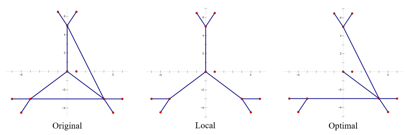
对于Minimum Degree Spanning Tree，同样的原图(Original)，寻找反例如下:

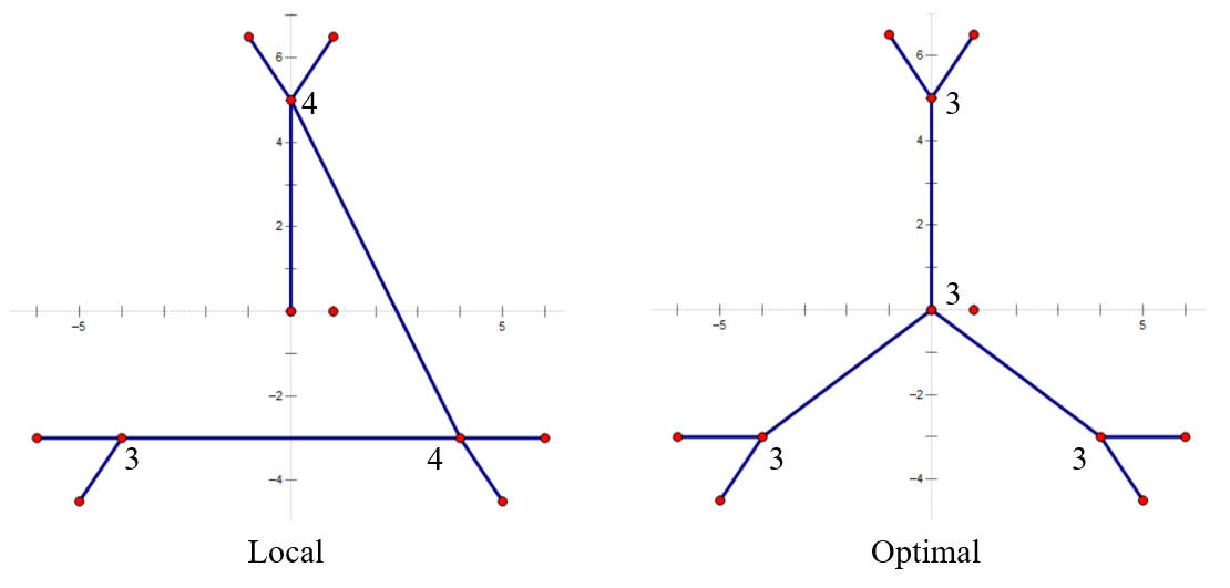
究其本质，最小生成树如果有更好的选择一定能交换，因为进行的正是边交换，直接影响的就是树的整体权值。另外两种树的性质则与顶点相关，不能直接影响，所以就寄了。
Q2-2. There are$n$jobs, and each job$j$has a processing time$t_{j}$. We will use a local search algorithm to partition the jobs into two groups A and B, where set A is assigned to machine$M_{1}$and set$\mathrm{B}$to$M_{2}$. The time needed to process all of the jobs on the two machines is$T_{1}=\sum_{j \in A} t_{j}, T_{2}=\sum_{j \in B} t_{j}$. The problem is to minimize$\left|T_{1}-T_{2}\right|$.

Local search: Start by assigning jobs$1, \ldots, n / 2$to$M_{1}$, and the rest to$M_{2}$.

The local moves are to move a single job from one machine to the other, and we only move a job if the move decreases the absolute difference in the processing times. Which of the following statement is true?

A. The problem is NP-hard and the local search algorithm will not terminate.

B. When there are many candidate jobs that can be moved to reduce the absolute difference, if we always move the job$j$with maximum$t_j$, then the local search terminates in at most$n$moves.

C. The local search algorithm always returns an optimal solution.

D. The local search algorithm always returns a local solution with$\frac{1}{2}T_1\leqslant T\leqslant 2T_1$.

B。

A，每次都减小，肯定会减无可减，那么一定会终止。NP-hard猜想应该是的，一共有$2^n$种状态。

B，一项被移到另一侧之后肯定不会再被移回来，因此最多移$n$次。

C，考虑$\{10,11,12,12,13,14\}=\{10,11,13\}+\{12,12,14\}$，可知无法移动了，但是显然最优解是$\{11,12,13\}+\{10,12,14\}$。

D，考虑$\{1,2,100\}=\{1,2\}+\{100\}$。
Q2-3. Max-cut problem: Given an undirected graph$G=(V, E)$with positive integer edge weights$w_{e}$, find a node partition$(A, B)$such that$w(A, B)$, the total weight of edges crossing the cut, is maximized. Let us define$S^{\prime}$be the neighbor of$S$such that$S^{\prime}$can be obtained from$S$by moving one node from$A$to$B$, or one from$B$to$A$. only choose a node which, when flipped, increases the cut value by at least$w(A, B) /|V|$. Then which of the following is true?

A. Upon the termination of the algorithm, the algorithm returns a cut$(A,B)$so that$2.5w(A,B)\geqslant w(A^∗, b^*)$, where$(A^∗ ,B^∗)$is an optimal partition.

B. The algorithm terminates after at most$O(\log|V|\log W)$flips, where$W$is the total weight of edges.

C. Upon the termination of the algorithm, the algorithm returns a cut$(A,B)$so that$2w(A,B)\geqslant w(A^∗, b^*)$.

D. The algorithm terminates after at most$O(|V|^2)$flips.

题目中给出条件，increase the cut value by at least w(A,B)/V,说明此时$\epsilon = 0.5$

根据定理，最后至多执行$n/\epsilon \ logW$次flip

最终结果满足，$w(A^*,B^*) < (2 + \epsilon)w(A,B)$