8. Dynamic Programming
约 3231 个字 149 行代码 预计阅读时间 18 分钟
7.1. 动态规划简介
-
动态规划的定义
动态规划(Dynamic Programming):简称 DP,是一种求解多阶段决策过程最优化问题的方法。在动态规划中,通过把原问题分解为相对简单的子问题,先求解子问题,再由子问题的解而得到原问题的解。
-
动态规划的核心思想
动态规划的核心思想:
- 把「原问题」分解为「若干个重叠的子问题」,每个子问题的求解过程都构成一个 「阶段」。在完成一个阶段的计算之后,动态规划方法才会执行下一个阶段的计算。
- 在求解子问题的过程中,按照「自顶向下的记忆化搜索方法」或者「自底向上的递推方法」求解出「子问题的解」,把结果存储在表格中,当需要再次求解此子问题时,直接从表格中查询该子问题的解,从而避免了大量的重复计算。
这看起来很像是分治算法,但动态规划与分治算法的不同点在于:
- 适用于动态规划求解的问题,在分解之后得到的子问题往往是相互联系的,会出现若干个重叠子问题。
使用动态规划方法会将这些重叠子问题的解保存到表格里,供随后的计算查询使用,从而避免大量的重复计算。
-
动态规划的简单例子
斐波那契数列:数列由 \(f(0) = 1,f(1) = 2\) 开始,后面的每一项数字都是前面两项数字的和。
通过公式 \(f(n) = f(n - 2) + f(n - 1)\),我们可以将原问题 \(f(n)\) 递归地划分为 \(f(n - 2)\) 和 \(f(n - 1)\) 这两个子问题。其对应的递归过程如下图所示:
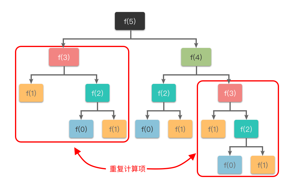
从图中可以看出:如果使用传统递归算法计算 \(f(5)\),需要先计算 \(f(3)\) 和 \(f(4)\),而在计算 \(f(4)\) 时还需要计算 \(f(3)\),这样 \(f(3)\) 就进行了多次计算。同理 \(f(0)\)、\(f(1)\)、\(f(2)\) 都进行了多次计算,从而导致了重复计算问题。
为了避免重复计算,我们可以使用动态规划中的「表格处理方法」来处理。
这里我们使用「自底向上的递推方法」求解出子问题 \(f(n - 2)\) 和 \(f(n - 1)\) 的解,然后把结果存储在表格中,供随后的计算查询使用。具体过程如下:
- 定义一个数组 \(dp\),用于记录斐波那契数列中的值。
- 初始化 \(dp[0] = 0,dp[1] = 1\)。
- 根据斐波那契数列的递推公式 \(f(n) = f(n - 1) + f(n - 2)\),从 \(dp(2)\) 开始递推计算斐波那契数列的每个数,直到计算出 \(dp(n)\)。
- 最后返回 \(dp(n)\) 即可得到第 \(n\) 项斐波那契数。
具体代码如下:
int Fibonacci(int N)
{
    int i, Last, NextToLast, Answer;
    if (N <= 1)
        return 1;
    Last = NextToLast = 1;
    /* F(0) = F(1) = 1 */
    for (i = 2; i <= N; i++)
    {
        Answer = Last + NextToLast;
        /* F(i) = F(i-1) + F(i-2) */
        NextToLast = Last;
        Last = Answer;
        /* update F(i-1) and F(i-2) */
    } /* end-for */
    return Answer;
}
这种使用缓存(哈希表、集合或数组)保存计算结果,从而避免子问题重复计算的方法,就是「动态规划算法」。
7.2. 动态规划的特征
究竟什么样的问题才可以使用动态规划算法解决呢?
首先,能够使用动态规划方法解决的问题必须满足以下三个特征:
- 最优子结构性质
- 重叠子问题性质
- 无后效性
7.2.1 最优子结构性质
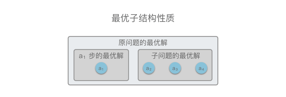
最优子结构:指的是一个问题的最优解包含其子问题的最优解。
举个例子,如下图所示,原问题 \(S = \lbrace a_1, a_2, a_3, a_4 \rbrace\),在 \(a_1\) 步我们选出一个当前最优解之后,问题就转换为求解子问题 \(S*{子问题} = \lbrace a_2, a_3, a_4 \rbrace\)。如果原问题 \(S\) 的最优解可以由「第 \(a_1\) 步得到的局部最优解」和「 \(S*{子问题}\) 的最优解」构成,则说明该问题满足最优子结构性质。
也就是说,如果原问题的最优解包含子问题的最优解,则说明该问题满足最优子结构性质。
7.2.2 重叠子问题性质
重叠子问题性质:指的是在求解子问题的过程中,有大量的子问题是重复的,一个子问题在下一阶段的决策中可能会被多次用到。如果有大量重复的子问题,那么只需要对其求解一次,然后用表格将结果存储下来,以后使用时可以直接查询,不需要再次求解。
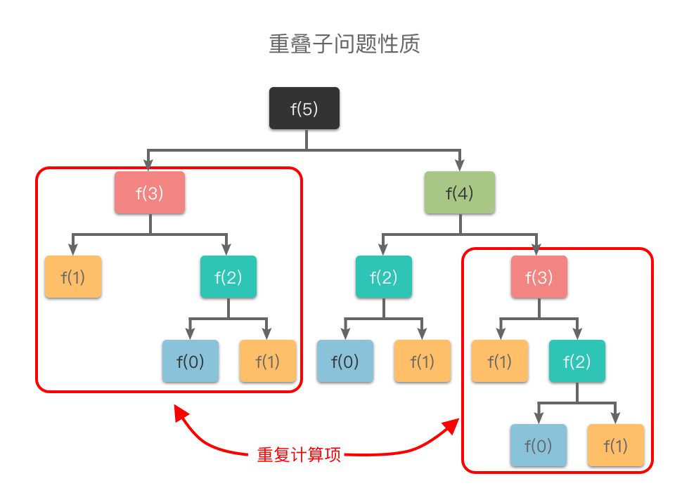
之前我们提到的「斐波那契数列」例子中,\(f(0)\)、\(f(1)\)、\(f(2)\)、\(f(3)\) 都进行了多次重复计算。动态规划算法利用了子问题重叠的性质,在第一次计算 \(f(0)\)、\(f(1)\)、\(f(2)\)、\(f(3)\) 时就将其结果存入表格,当再次使用时可以直接查询,无需再次求解,从而提升效率。
7.2.3 无后效性
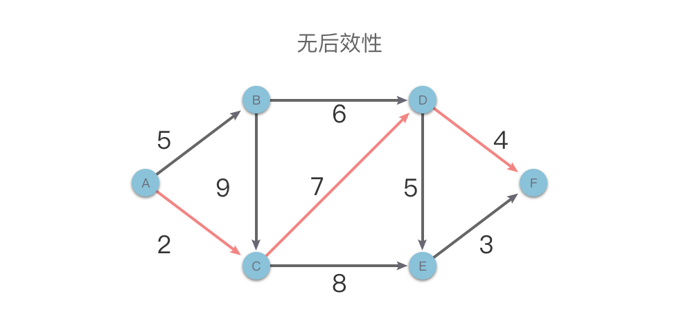
无后效性:指的是子问题的解(状态值)只与之前阶段有关,而与后面阶段无关。当前阶段的若干状态值一旦确定,就不再改变,
不会再受到后续阶段决策的影响。
也就是说,一旦某一个子问题的求解结果确定以后,就不会再被修改。
举个例子,下图是一个有向无环带权图,我们在求解从 \(A\) 点到 \(F\) 点的最短路径问题时,假设当前已知从 \(A\) 点到 \(D\) 点的最短路径(\(2 + 7 = 11\))。那么无论之后的路径如何选择,都不会影响之前从 \(A\) 点到 \(D\) 点的最短路径长度。这就是「无后效性」。
而如果一个问题具有「后效性」,则可能需要先将其转化或者逆向求解来消除后效性,然后才可以使用动态规划算法。
7.3. 动态规划的基本思路
如下图所示,我们在使用动态规划方法解决某些最优化问题时,可以将解决问题的过程按照一定顺序(时间顺序、空间顺序或其他顺序)分解为若干个相互联系的「阶段」。然后按照顺序对每一个阶段做出「决策」,这个决策既决定了本阶段的效益,也决定了下一阶段的初始状态。依次做完每个阶段的决策之后,就得到了一个整个问题的决策序列。
这样就将一个原问题分解为了一系列的子问题,再通过逐步求解从而获得最终结果。
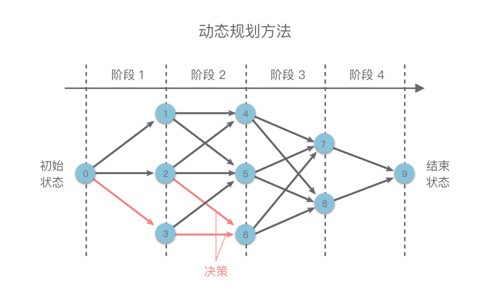
这种前后关联、具有链状结构的多阶段进行决策的问题也叫做「多阶段决策问题」。
通常我们使用动态规划方法来解决问题的基本思路如下:
- 划分阶段:将原问题按顺序(时间顺序、空间顺序或其他顺序)分解为若干个相互联系的「阶段」。划分后的阶段⼀定是有序或可排序的,否则问题⽆法求解。
- 这里的「阶段」指的是⼦问题的求解过程。每个⼦问题的求解过程都构成⼀个「阶段」,在完成前⼀阶段的求解后才会进⾏后⼀阶段的求解。
- 定义状态:将和子问题相关的某些变量(位置、数量、体积、空间等等)作为一个「状态」表示出来。状态的选择要满⾜⽆后效性。
- 一个「状态」对应一个或多个子问题,所谓某个「状态」下的值,指的就是这个「状态」所对应的子问题的解。
- 状态转移:根据「上一阶段的状态」和「该状态下所能做出的决策」,推导出「下一阶段的状态」。或者说根据相邻两个阶段各个状态之间的关系,确定决策,然后推导出状态间的相互转移方式(即「状态转移方程」)。
- 初始条件和边界条件:根据问题描述、状态定义和状态转移方程,确定初始条件和边界条件。
- 最终结果:确定问题的求解目标,然后按照一定顺序求解每一个阶段的问题。最后根据状态转移方程的递推结果,确定最终结果。
7.4. 动态规划的应用
7.4.1 Ordering Matrix Multiplication
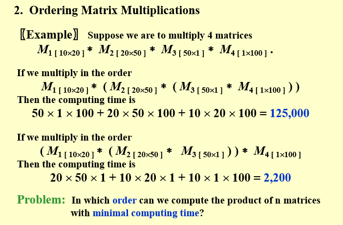
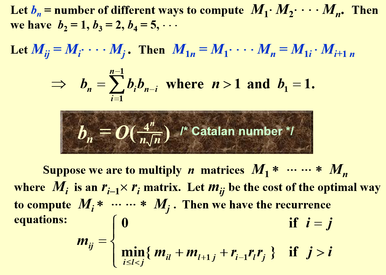
令\(b_n\)表示计算\(M_1 \cdot M_2 \cdots M_n\)不同方法的数量
我们能够将\(M_1 \cdot M_2 \cdots M_n\)分成两部分,记\(M_{ij} = M_i \cdots M_j\)
那么只需要在矩阵序列中切一刀,就得到两个矩阵序列
此时得到\(b_n\)的递推关系
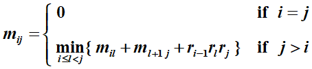
接下来正式计算\(M_1 \cdot M_2 \cdots M_n\),\(M_i\)是一个\(r_{i-1}\times r_i\) 的矩阵. 用\(m_{ij}\)表示计算\(M_{ij}\)的结果
最后转化为 Mil, Mlj, 以及两个矩阵的相乘
// 利用动态规划,先计算 m11,m22,....mNN
// 再向上计算 m12,m23,...,逐层向上
int Optmatrix(vector<int> &p, vector<vector<int>> &m, int n)
{
    int i, j, k;
    for(i = 1; i <= n; i++) m[i][i] = 0;
    // 接下来依次计算m[i][j]的最小值
    for(i = 1; i <= n -1; i++)
    {
        // 计算m[i][j]的最小值
        for(j = 1; j <= n - i; j++)
        {
            int min = MAX;
            for(k = j; k <= j + i - 1; k++)
            {
                m[j][j+i] = m[j][k] + m[k+1][j+i] + p[j-1]*p[k]*p[j+i];
                if(m[j][j+i] < min) min = m[j][j+i];
            }
            m[j][j+i] = min;
        }
    }
    return m[1][n];
}
7.4.2 Optimal Binary Search Tree
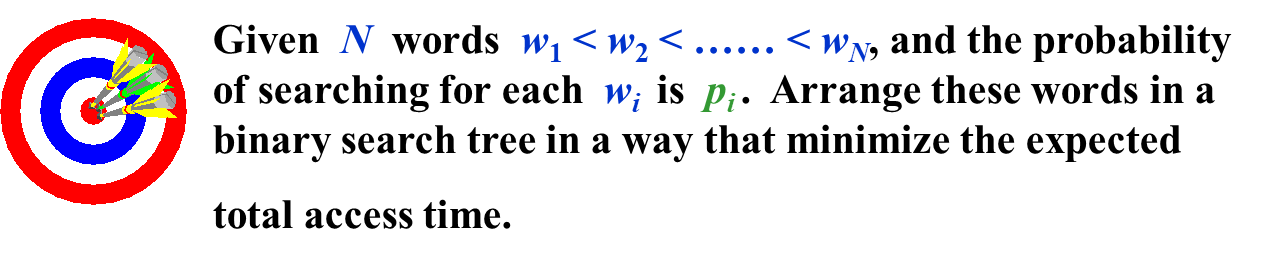
\(T(N) = \sum_{i =1}^N p_i(1+d_i)\)
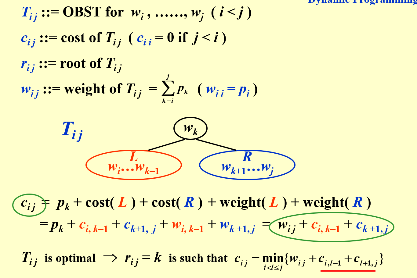
依然是拆分成两部分
\(C_{ij} = p_k + cost(L) + cost(R) + weight(L) + weight(R)\)
\(C_{ij} = p_k + C_{i,k-1}+C_{k+1,j} + W_{i.k-1} + W_{k+1,j} = C_{i,k-1} + C_{k+1,j} + W_{ij}\)
此处添加weight(L)和weight(R)的原因是,L和R成为子树之后,所有的深度都会加1,利用pi(1+di),可知子树所有结点的权重需要累加
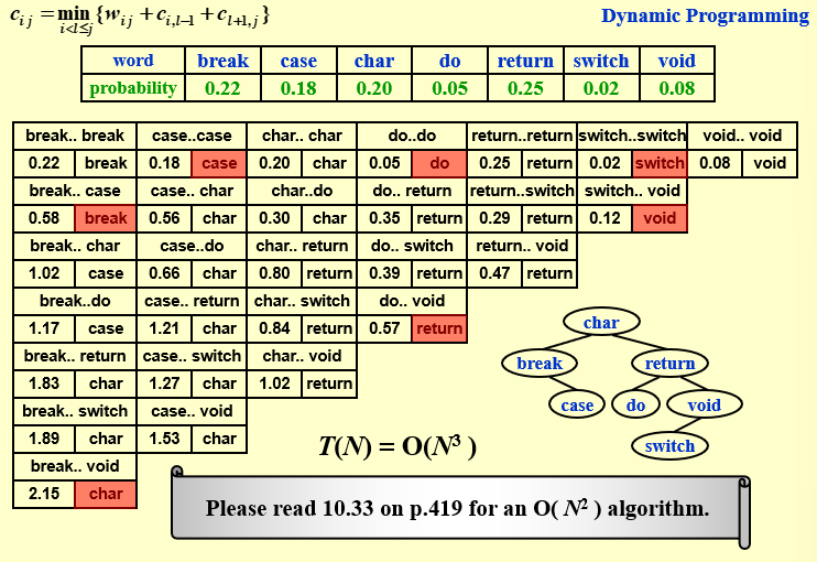
从底到顶,先计算长度为1的最小值,在利用长度为1的最小值,计算长度为2的最小值
第一行长度为1,就是本身的weight
第二行长度为2,\(min = (w_ij + min(w_i,w_j))\)
第三行长度为3,以break…char为例
- break为根结点,break-(case..char) = 0.6 + 0.56 = 1.16
- case为根结点, break - case -char = 0.6 + 0.22 + 0.20 = 1.02
- char为根结点, (break..case) char = 0.6 + 0.58 = 1.18
第四行长度为4,以break…do为例
- break为根结点,break-(case … do) = 0.65 + 0.66 = 1.31
- case 为根结点, break-case-(char..do) = 0.65 + 0.22 + 0.30 = 1.17
- char 为根结点, (break..case) - char -do = 0.65 + 0.58 + 0.05 = 1.28
- do为根结点,(break…char) - do = 0.65 + 1.02 = 1.67
// Dynamic programming function to find the minimum cost
double DP(vector<double> &weight, vector<vector<double>> &cost, int n)
{
    int i, j, k;
    // Initializing the diagonal of the cost matrix
    for(i = 1; i <= n; i++) cost[i][i] = weight[i];

    // Filling up the cost matrix using dynamic programming
    for(int len = 1; len <= n-1; len++)
    {
        for(i = 1; i <= n-len; i++)
        {
            j = i + len;
            double mincost = 1e9;  // Initializing mincost to a very large value

            // Checking for the base case when len = 1
            if(len == 1)
            {
                cost[i][j] = SumWeight(weight, i, j) + min(weight[i], weight[j]);
            }
            else
            {
                // Iterating through possible partitions and finding the minimum cost
                for(k = i; k < j; k++)
                {
                    double temp = cost[i][k-1] + cost[k+1][j] + SumWeight(weight, i, j);
                    if(temp < mincost) mincost = temp;
                }
                cost[i][j] = mincost;  // Assigning the minimum cost for this range
            }
        }
    }
    return cost[1][n];  // Returning the minimum cost for the entire range
}
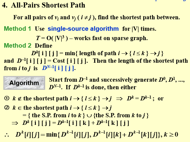
7.4.3 All-Pairs Shortest Path
-
迪杰斯特拉算法(执行n次)
-
动态规划(也就是弗洛伊德算法)。start from \(D^{-1}\),依次计算生成\(D^0,D^1,....D^n\)
能够存在负边,但是不能存在负环
/* A[ ] contains the adjacency matrix with A[ i ][ i ] = 0 */
/* D[ ] contains the values of the shortest path */
/* N is the number of vertices */
/* A negative cycle exists iff D[ i ][ i ] < 0 */
void AllPairs(TwoDimArray A, TwoDimArray D, int N)
{
    int i, j, k;
    for (i = 0; i < N; i++) /* Initialize D */
        for (j = 0; j < N; j++)
            D[i][j] = A[i][j];
    for (k = 0; k < N; k++) /* add one vertex k into the path */
        for (i = 0; i < N; i++)
            for (j = 0; j < N; j++)
                if (D[i][k] + D[k][j] < D[i][j])
                    /* Update shortest path */
                    D[i][j] = D[i][k] + D[k][j];
}
7.4.4 Product Assembly
-
暴力法求解

-
动态规划
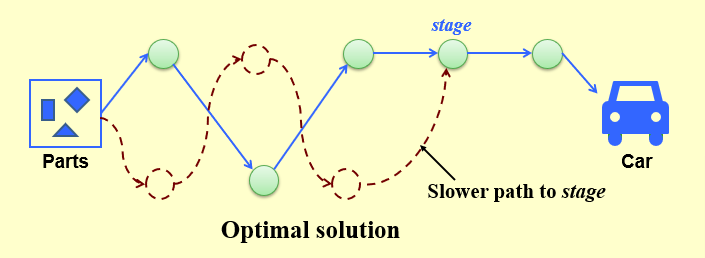
An optimal path to stage is based on an optimal path to stage–1
当前的最优解,依赖于前一步的最优解
同一条产品线继续或者从另外一条线进行转移
O( N ) time + O( N ) space
f[0][0]=0; L[0][0]=0;
f[1][0]=0; L[1][0]=0;
for(stage=1; stage<=n; stage++){
    for(line=0; line<=1; line++){
    f_stay = f[  line][stage-1] + t_process[  line][stage-1];
    f_move = f[1-line][stage-1] + t_transit[1-line][stage-1];
    if (f_stay<f_move){
        f[line][stage] = f_stay;
        L[line][stage] = line;
    }
    else {
        f[line][stage] = f_move;
        L[line][stage] = 1-line;
    }
    }
}
7.5 习题集
-
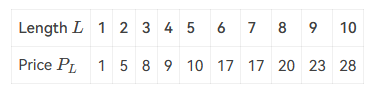
Rod-cutting Problem: Given a rod of total length \(N\) inches and a table of selling prices \(P_L\) for lengths \(L = 1, 2, \cdots , M\). You are asked to find the maximum revenue \(R_N\) obtainable by cutting up the rod and selling the pieces. For example, based on the following table of prices, if we are to sell an 8-inch rod, the optimal solution is to cut it into two pieces of lengths 2 and 6, which produces revenue \(R_8 = P_2 +P_6 = 5+17 = 22\). And if we are to sell a 3-inch rod, the best way is not to cut it at all.
Which one of the following statements is FALSE?
-
A. This problem can be solved by dynamic programming
-
B. The time complexity of this algorithm is \(O(N^2)\)
-
C. If \(N\le M\), we have \(R_N = \max \lbrace P_N , \max_{1\le i < N} \lbrace R_i + R_{N-i} \rbrace \rbrace\)
-
D. If \(N>M\), we have \(R_N = \max_{1\le i < N} \lbrace R_i + R_{N-M} \rbrace\)
B:\[ \begin{aligned} &R1 = P1\\ &R2 = max\{P2, R1 + P1\}\\ &R3 = max\{P3, P2 + R1, P1 + R2\}\\ &....\\ &计算R_n需要 1 + 2 + 3 + 4 + ... + n 步 \end{aligned} \]D:\(R_N = max_{1<= i < N}\{R_i + R_{N - i} \}\) -
-
In dynamic programming, we derive a recurrence relation for the solution to one subproblem in terms of solutions to other subproblems. To turn this relation into a bottom up dynamic programming algorithm, we need an order to fill in the solution cells in a table, such that all needed subproblems are solved before solving a subproblem. Among the following relations, which one is impossible to be computed?
-
A. \(A(i, j) = min (A(i-1,j), A(i,j-1), A(i-1,j-1))\)
-
B. \(A(i, j) = F(A(min\{i, j\} - 1, min\{i, j\} - 1), A(max\{i, j\} - 1, max\{i, j\} -1))\)
-
C. \(A(i, j) = F(A(i, j -1), A(i - 1, j - 1), A(i - 1, j + 1))\)
-
D. \(A(i,j) = F(A(i-2, j-2), A(i+2,j+2))\)
要实现动态规划,讲究一个先来后到,显然D的计算顺序有误对于C,可以 for i in 0 to n: for j in 0 to n 先计算(i - 1, )所有的组合,这样 (i - 1, j + 1)的组合也就提前计算了
-
-
Given a recurrence equation \(f_{i,j,k} =f_{i,j+1,k}+\min_{0 \le l \le k}\{f_{i-1,j,l}+w_{j,l}\}\). To solve this equation in an iterative way, we cannot fill up a table as follows:
-
A. for k in 0 to n: for i in 0 to n: for j in n to 0
-
B. for i in 0 to n: for j in 0 to n: for k in 0 to n
-
C. for i in 0 to n: for j in n to 0: for k in n to 0
-
D. for i in 0 to n: for j in n to 0: for k in 0 to n
j 不能增序算,因为 \(f_{i,j,k}\) 依赖于 \(f_{i,j+1,k}\)。
-
-
If a problem can be solved by dynamic programming, it must be solved in polynomial time.
F0-1背包问题可以用DP解,但是复杂度不是多项式的, 原因是输入的数据不是多项式的
背包问题
-
背包问题的背景:
给定背包的承重W, 一堆物品的重量weight[]和价值value[],求背包能装入物品的最大总value
-
背包问题的解法:
定义一个二维数组dp
其中 $dp[i] [j] $表示:从前 i 件物品中找出一些放入背包,在总重不超过承重W的情况下,能达到的最大value。
第 i 件物品重量为 weight[i],价值为 value[i],根据第 i 件物品是否添加到背包中,可以分两种情况讨论:
- 第 i 件物品的重量超过背包承重,即 weight[i] > j。此时就算拿出背包中的所有物品也无法放下,所以它不可能被放入背包,因此有:
dp[i][j] = dp[i-1][j] - 第 i 件物品可以添加到背包中(可能拿出一些已有物品)。此时也可以有放入与不放入两种情况,应取value更大的那种。
- 若不放入,有:
dp[i][j] = dp[i-1][j] - 若放入,情况变为从某个状态下加入第i件物品并达到dp[i][j]结果,可知前一状态时的背包承重应为 j-weight[i]。因此有:
dp[i][j] = dp[i-1][ j-weight[i] ] + value[i]。
- 若不放入,有:
- 第 i 件物品的重量超过背包承重,即 weight[i] > j。此时就算拿出背包中的所有物品也无法放下,所以它不可能被放入背包,因此有:
-
得到递推式:
dp[i][j] = max(dp[i-1][j], dp[i-1][j-weight[i]] + value[i])
```cpp
int dp[W];
memset(dp, 0, sizeof(dp));
for(int i = 0; i < n; i++)
{
    for(int j =  W; j >= 1; j--)
    {
        if(j >= weight[i])
        {
            dp[j] = max(dp[j], dp[j - weight[i]] + value[i]);
        }
    }
}
return dp[W];
```
For problem i, Bob will need time[i] to solve it and obtains the corresponding score[i], or he may choose not to solve it at all. Bob will be happy when he obtains a total score no less than happy_score. You are supposed to find the minimum time needed for Bob to be happy. The function need_time must return the minimum time, or -1 if it is impossible for Bob to obtain a score no less than happy_score.
Format of function:
int need_time(const int time[], const int score[], int happy_score, int n);
Here n (1≤n≤ MAXN) is the number of problems;
happy_score (1≤ happy_score ≤ MAXS) is the minimum score for Bob to be happy;
time[] is the array to store time[i] (1≤time[i]≤100) which is the time to solve problem i;
score[] is the array to store score[i] (1≤score[i]≤100) which is the score Bob gets for solving problem i.
PTA的题目要求是:
1.开心值总和 >= happy_score 2.所花时间总和最少
上述的背包问题不再适用恰好是其反面
从逆向思维出发:要求score总和小于 sum_score - happy_score,并且总time最大,符合背包的假设.最后只需要用sum_time-逆向时间的最大值即可得到正向的最小时间
int need_time(const int time[], const int score[], int happy_score, int n)
{
    // 背包问题
    int sum_score = 0;
    int sum_time = 0;
    for (int i = 0; i < n; i++)
    {
        sum_score += score[i];
        sum_time += time[i];
    }
    if(sum_score < happy_score) return -1;

    // 我们要计算,不达到happy_score的情况下,最多需要多少时间
    // 这样就可以用总时间减去这个时间,就是最少时间
    int dp[sum_score];
    memset(dp, 0, sizeof(dp));
    for(int i = 0; i < n; i++)
    {
        for(int j = sum_score - happy_score; j >= score[i]; j--)
        {
            dp[j] = dp[j] > dp[j - score[i]] + time[i] ? dp[j] : dp[j - score[i]] + time[i];
        }
    }
    return sum_time - dp[sum_score - happy_score];
}