12. Query Optimization

约 5087 个字 10 行代码 预计阅读时间 26 分钟

Abstract

• Introduction
• Transformation of Relational Expressions
• Statistical Information for Cost Estimation
• Cost-based Optimization
• Dynamic Programming for Choosing Evaluation Plans
• Nested Subqueries
• Materialized Views
• Advanced Topics in Query Optimization

12.1 Introduction

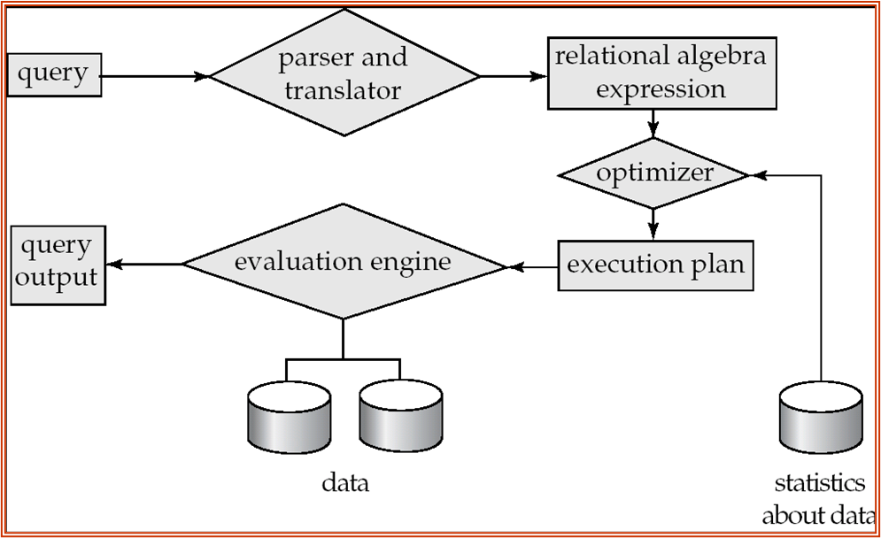
Alternative ways of evaluating a given query

• Equivalent expressions

  逻辑优化：关系代数表达式（尽量先做选择，投影）Transformation Base Optimization

• Different algorithms for each operation

  物理层面：每个算子选择不同的算法 Cost Based Optimization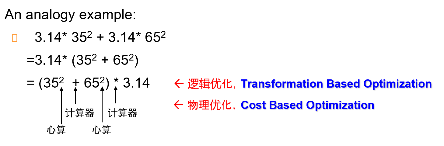

  
  

Estimation of plan cost based on: 计划成本估算

• Statistical information about relations. Examples: number of tuples, number of distinct values for an attribute

  有关关系的统计信息。示例：元组数、属性的非重复值数

• Statistics estimation for intermediate results（Cardinality Estimation） to compute cost of complex expressions

  中间结果的统计估计（基数估计）用于计算复杂表达式的成本

  估计中间结果的大小 现在有基于深度学习的估计方法

• Cost formulae for algorithms, computed using statistics

  算法的成本公式，使用统计数据计算

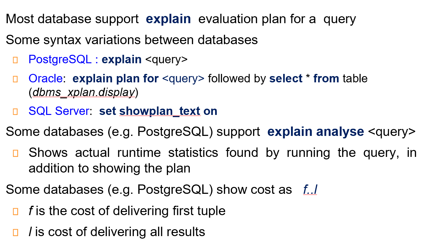
关系数据库里可以用查看执行计划。（view query evaluation plan）

12.2 Generating Equivalent Expressions

Two relational algebra expressions are said to be equivalent if the two expressions generate the same set of tuples on every legal database instance

等价关系代数表达式：

两个关系代数表达式等价是指：形式不同，但产生的OUTPUT是完全相同的。

12.2.1 Equivalence Rules

An equivalence rule says that expressions of two forms are equivalent

等价规则表示两种形式的表达式是等价的

Can replace expression of first form by second, or vice versa

可以用第二种形式替换第一种形式的表达，反之亦然

• selection

  

  1. 可以把算子拆分

     如果某些属性有索引，那么可以先拆分，在索引 select 之后再执行其他算子.

     如果有复合索引，可以逆向进行

  2. 算子可交换 先执行有索引的算子。

  3. 投影的属性可以只保留最后一次的

  4. 选择算子可以和（笛卡尔积和连接）结合

• join
  

  

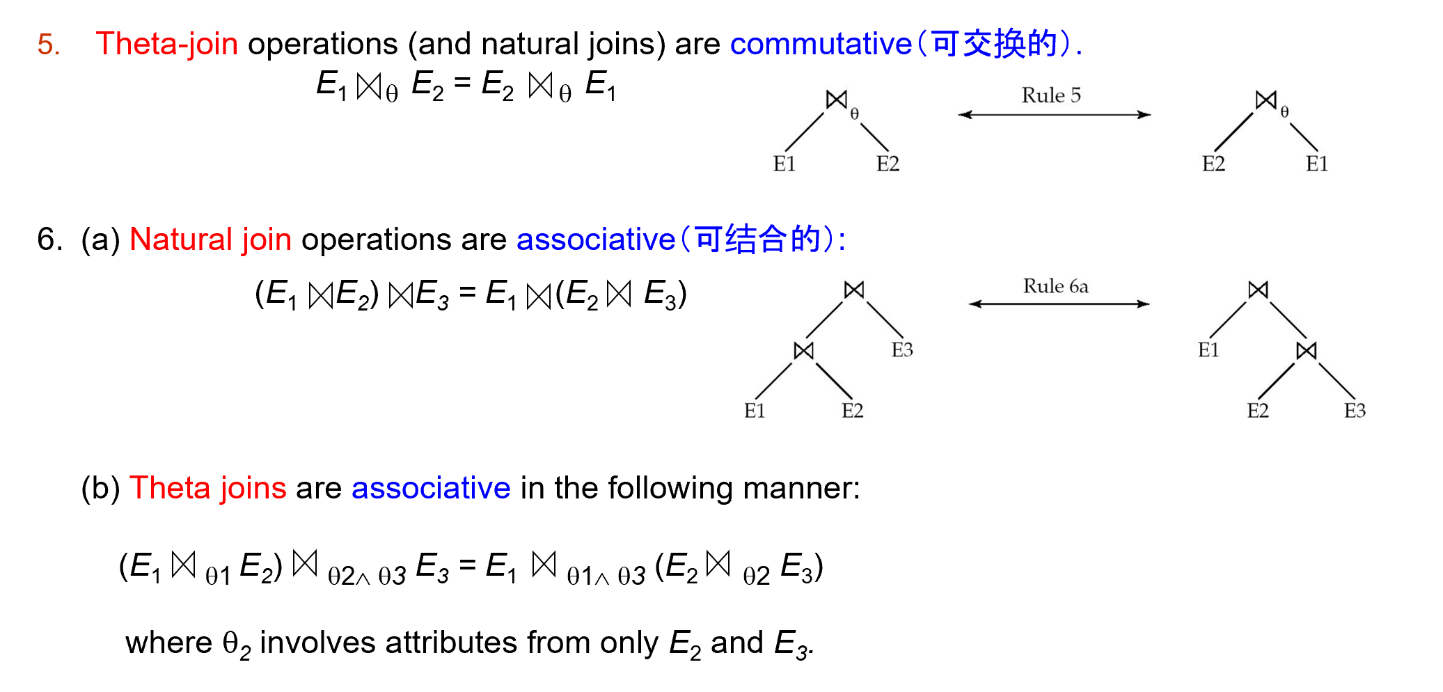
  自然连接是结合的（先连接中间结果小的）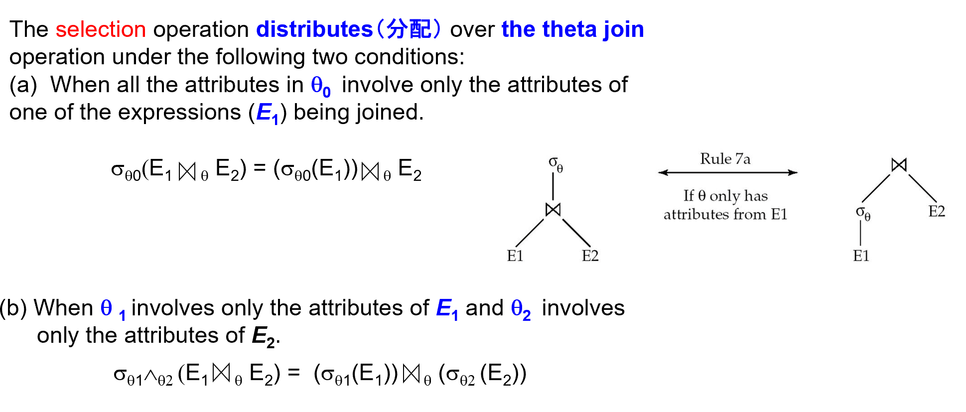

  

  如果选择算子只和一个关系有关，那么我们可以先执行选择。（选择算子要早进行，推到叶子上）

• projection

  

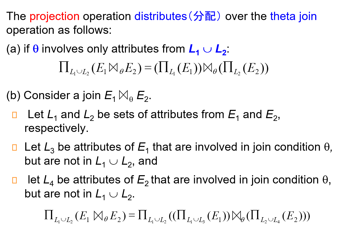
  这体现的是：投影运算也应该尽量先做。投影运算与选择运算都能降低结果的规模。

  • 先做投影再进行连接（有前提条件，\(\theta\)不能涉及到L1和L2之外的属性）。

  • 如果连接要用到投影后不保留的属性，我们在第一次投影时要把连接用的属性也保留下来。

• set operation

  

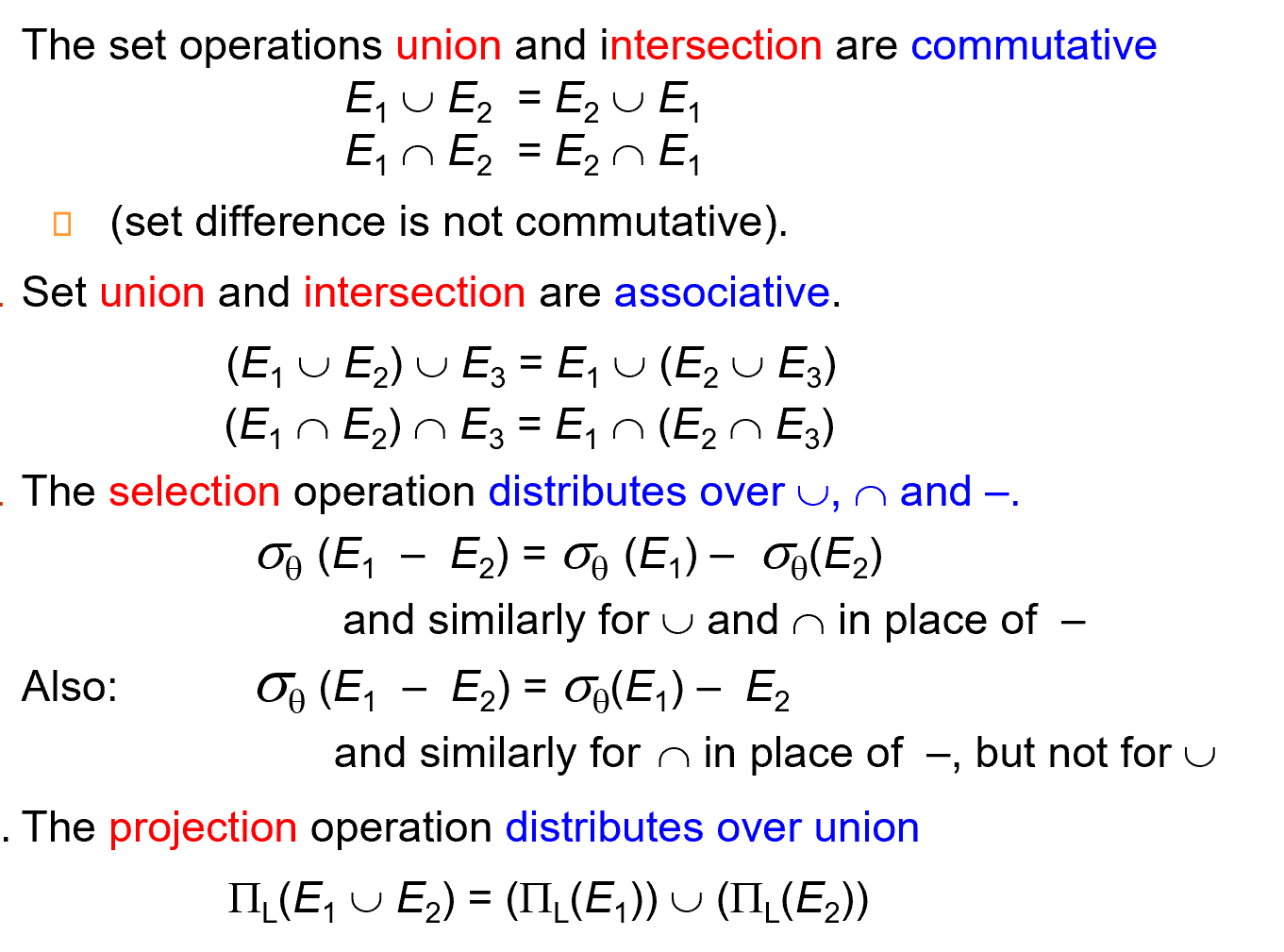
  针对集合的选择操作是可分配的 $$ \sigma_\theta(E1- E2) = \sigma_\theta(E1) - \sigma_\theta(E2)\ \sigma_\theta(E1 \cap E2) = \sigma_\theta(E1) \cap \sigma_\theta(E2)\ \sigma_\theta(E1 \cup E2) = \sigma_\theta(E1) \cup \sigma_\theta(E2)\ $$ 对于减法：\(E1-E2\)表示E1有但是E2没有的部分，然后再对这一部分进行\(\theta\)条件的选择，得到结果。假设E1和E2存在同时满足\(\theta\)条件的元素，在左边显然E1-E2就已经删除该元素，右边同理，共有元素删除。 $$ \sigma_\theta(E1- E2) = \sigma_\theta(E1) - E2 \ \sigma_\theta(E1 \cap E2) = \sigma_\theta(E1) \cap E2 \ \sigma_\theta(E1 \cup E2) != \sigma_\theta(E1) \cup E2\ $$ 注意此处的减法差集，可以理解为放缩为条件更强的式子，\(\sigma_\theta(E1)\)有但是E2没有的元素一定属于\(\sigma_\theta(E1)\)有，\(\sigma_\theta(E2)\)没有的集合

  集合的并对投影操作可分配

• other

  

  分组操作和选择操作可交换

  全连接的操作的可交换性

  选择操作对左右外部连接可分配

12.2.2 Enumeration of Equivalent Expressions

• Repeat

  • apply all applicable equivalence rules on every subexpression of every equivalent expression found so far

    对目前找到的每个等价表达式的每个子表达式应用所有适用的“等价规则”

  • add newly generated expressions to the set of equivalent expressions

    将新生成的表达式添加到等效表达式集中

• Until no new equivalent expressions are generated above

可以这样找到所有的等价表达式。

但是实际中我们基于一些经验规则进行启发式的优化

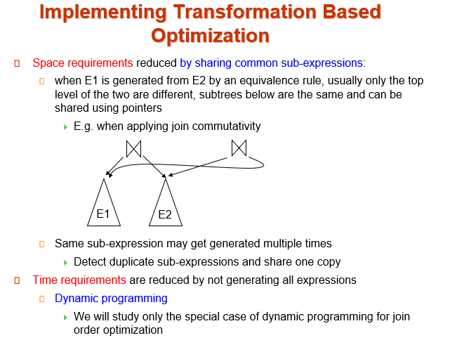
• 减少空间需求：共享相同的子表达式

  例如：连接的交换律

• 减少时间需求：使用动态规划

  每一次只考虑最优子序列的组合（长序列分为两个子序列）

12.3 Statistics for Cost Estimation

代价估算需要统计信息

• \(n_r\): number of tuples in a relation r.

  关系 r 中的元组数

• \(b_r\): number of blocks containing tuples of r.

  关系r的block块数

• \(l_r\): size of a tuple of r.

  关系r一个元组的大小

• \(f_r\): blocking factor of r — i.e., the number of tuples of r that fit into one block.

  一个块可以放多少个元组

• \(V(A, r)\): number of distinct values that appear in r for attribute A; same as the size of \(\Pi(r)\).

  关系 r 中某个属性A不同的值的个数。这也等价于对关系r中属性A进行投影，得到的结果集合大小。

• If tuples of r are stored together physically（存放是连续的） in a file, then: \(b_r = \lceil \dfrac{n_r}{f_r}\rceil\)

• Histograms

Example "attribute age of relation person"

Equi-Width Equi-Depth

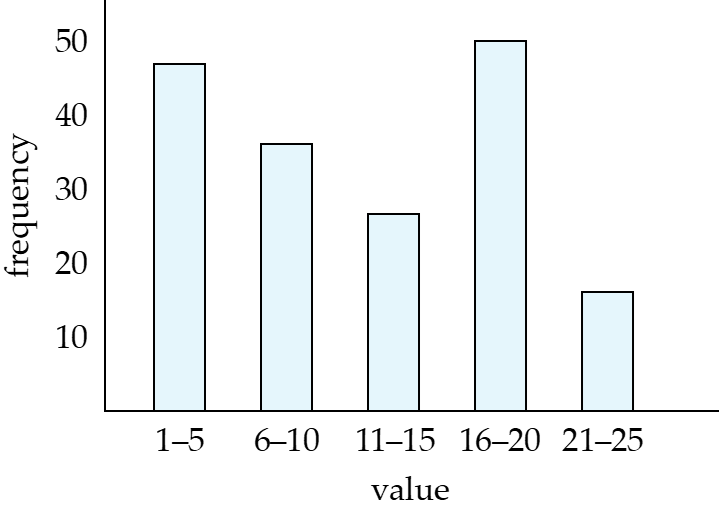
一般来说，对于一个关系 r 中的属性A，它又V(A,r)个不同的值，希望能用直方图表示这些不同的值分别有多少个元组。这样查询时，根据查询的范围，能够知道查询的结果的规模有多大。

但是我们往往没有直方图，对于每一个不同的值，采取平均分配的估计方式。也就是说，对于每一个值，估计表中存在\(n_r/V(A,r)\)个元组对应

12.3.1 Selection Size Estimation

中间结果

• \(\sigma_{A=v}(r)\)

\(n_r / V(A,r)\) : number of records that will satisfy the selection.

这样的估算基于值是平均分布的

• 若选择的这个属性A的这个值v不是key，那么就用总元组数除以这个属性的不同值的个数进行估计；

• 如果选择的这个属性A是key，那么估算为1。

• \(\sigma_{A\leq v}(r)\)

  • Let \(c\) denote the estimated number of tuples satisfying the condition.

  • \(c = 0\) if \(v < \min(A,r)\)

  • \(c = n_r\cdot \dfrac{v-\min(A,r)}{\max(A,r) - \min (A,r)}\) record总数 * 比例

  • In absence of statistical information c is assumed to be \(n_r / 2\)(

  假如数据库没有维护max或者min这些信息，只能将所有的小于等于操作或者大于等于操作得到的结果，估算为\(n_r/2\)了。

注意此处的OR运算(析取)，转化为AND操作（合取），要求各条件独立互不干扰。

至少满足一个条件转化为一个条件都不满足 $$ \theta_1 or \theta_2 = \neg((\neg \theta_1) and (\neg \theta_2)) $$

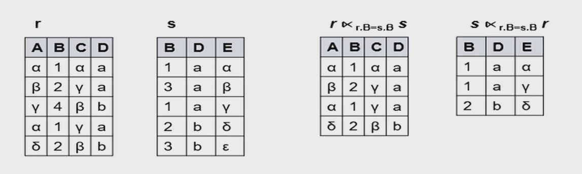
12.3.2 Estimation of the Size of Joins

The Cartesian product \(r \times s\) contains \(n_r\cdot n_s\) tuples; each tuple occupies \(s_r + s_s\) bytes.

• \(R \cap S = \emptyset\)

没有公共属性，自然连接\(r \bowtie s\)等价于 \(r\times s\)

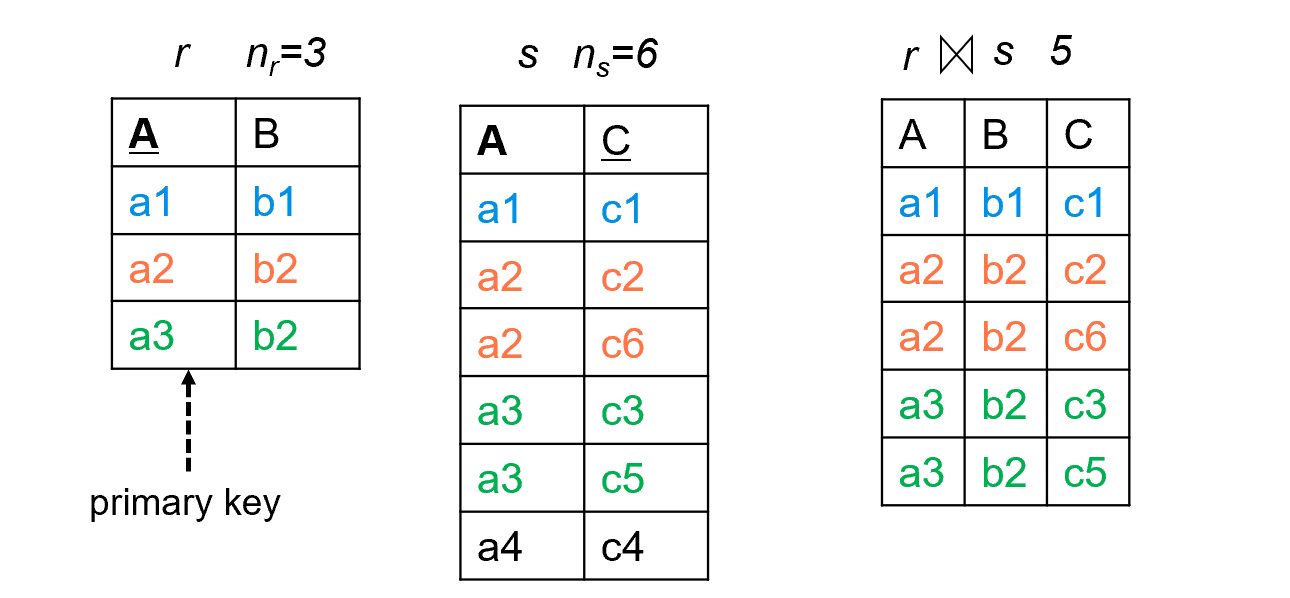
• \(R \cap S\) is a key for \(R\), then a tuple of \(s\) will join with at most one tuple from \(r\)

  (the number of tuples in \(r \bowtie s) \leq n_s\)

  从关系S的角度进行理解，连接用的属性为R的key，显然该属性不同的值在关系R中仅能出现一次，又因为该属性不一定是S的key，所以S中会出现多个相同的值，从而导致连接之后的元组个数\(\leq n_s\)

  

• If \(R \cap S\) in S is a foreign key in S referencing R, then the number of tuples in \(r\bowtie s\) = the number of tuples in s.

  foreign关系， a foreign key in S referencing R，说明连接用的属性不仅是R的key，同时任何出现在S中该属性的值都出现在R中，所以连接之后的元组数量为\(n_s\)

• If \(R \cap S = \{A\}\) is not a key for R or S.

  假如连接的属性不是某一个表的key

  \(n_r * \dfrac{n_s}{V(A,s)}, n_s * \dfrac{n_r}{V(A,r)}\).

  以第二个为例子，站在 s 的角度，\(\dfrac{n_r}{V(A,r)}\)表示关系 r 中属性A的每一个值对应有多少各记录，每一个 s 可以和属性A中每一个value对应的记录的平均值连接。

  因为有时候关系r中的一个元组对应属性值在s中没有出现，就会导致连接不上的情况，会导致估算结果偏大，所以通常我们取二者中的较小值。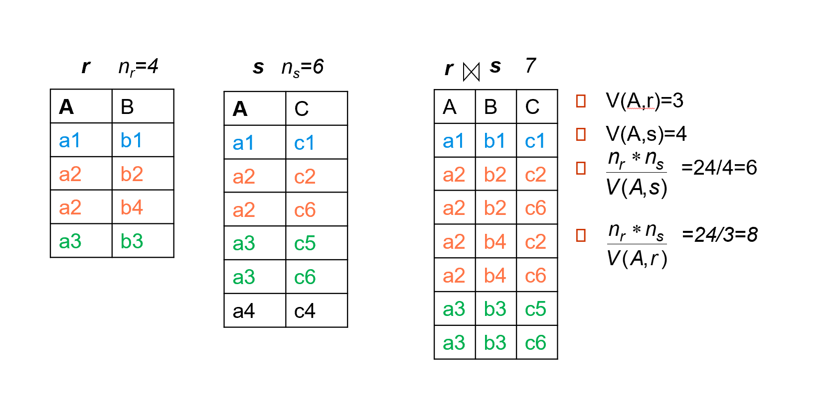

  

  

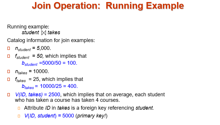
  此处V(ID,takes) = 2500， 表示在take关系中ID不同的value值的数量为2500，同时takes关系表中一共有10000个元组，说明上课的同学中平均每个同学上四门课

  ID是student关系中的primary key，所以student关系表中有多少元组，ID的value数量就有多少。因此V(ID,student) = n_student = 5000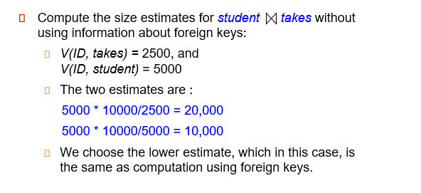

  

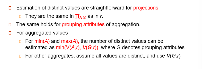
12.2.3 Size Estimation for Other Operations

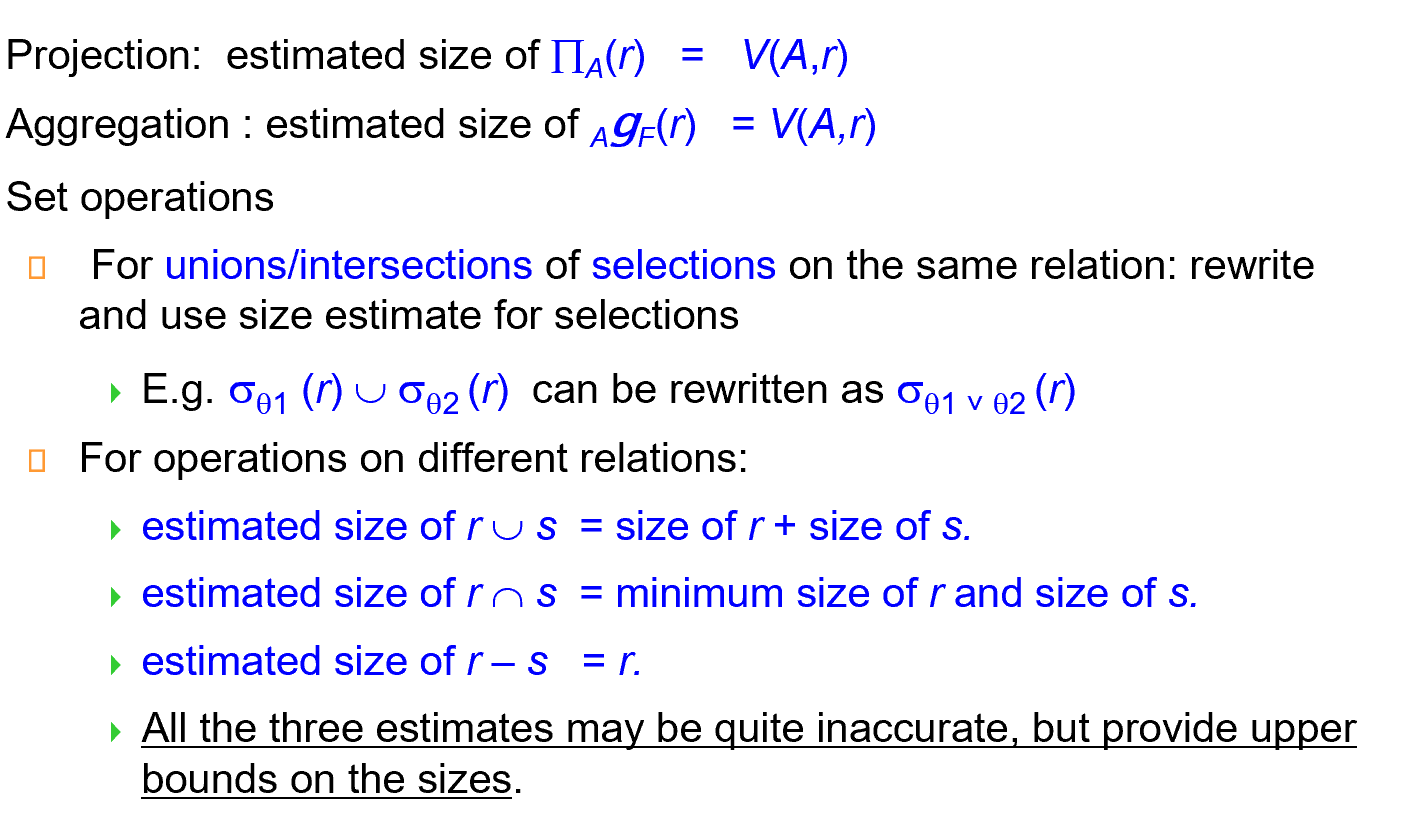
1. 投影：estimated size of \(\prod_A(r) = V(A,r)\)

2. 分组：在选定分组的基础上执行聚合函数，显然聚合函数根据输入的值只能得到一个结果，所以最优元组的数量为属性A中value的数量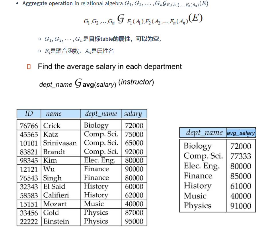

   

3. 对集合大小上下限的估算

   虽然不够精确，但是提供了上界。对于 - 操作，r - s 表示选取的是 r 有但是 s 没有的value，显然最大的size 为r

   

4. 对于外部自然连接的代价估算

   

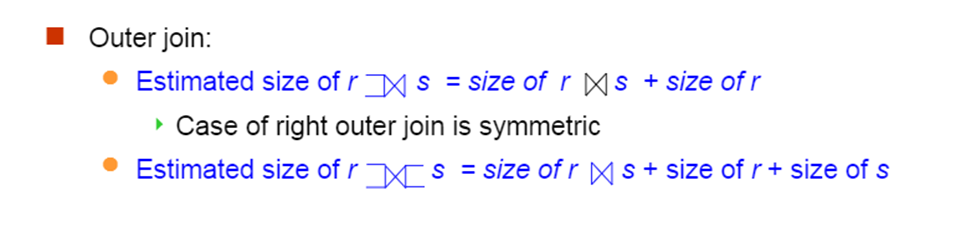
   外部连接比自然连接多出的是：假如是左外部连接，那么左边的关系没有连接上的部分，也要放入到结果集合中。因此结果集合的上限估算，就再加上r的元组个数。

12.2.4 Estimation of Number of Distinct Values

对于中间结果，在某个属性上不同值的个数

例如，估算下面这个选择操作中间结果在A属性上不同值的个数：

Selections \(\sigma_\theta(r)\), estimate \(V(A,\sigma_\theta(r))\) ****

• If \(\theta\) forces A to take a specified value, \(V(A,\sigma_\theta(r))=1\)

  e.g., A = 3

• If \(\theta\) forces A to take on one of a specified set of values: \(V(A,\sigma_\theta(r))=\) number of specified values

  e.g., (A = 1 V A = 3 V A = 4)

• If the selection condition \(\theta\) is of the form A op v, \(V(A,\sigma_\theta(r))=V(A,r)*s\)

  利用选择率 s 计算

• In all the other cases, use approx1imate estimate: \(V(A,\sigma_\theta(r))=\min(V(A,r), n_{\sigma_\theta(r)})\)

  原来未筛选的表在A属性上不同值的个数，和选择出来的结果条目的个数取最小值。

估算下面这个连接操作中间结果在A属性（可能是组合属性）上不同值的个数：

joins \(r\bowtie s\), estimate \(V(A,r\bowtie s)\)

• If all attributes in A are from r, the estimated \(V(A,r\bowtie s)=\min(V(A,r), n_{r\bowtie s})\)

• If A contains attributes A1 from r and A2 from s, then estimated

若A属性中包括属于r的属性集合A1，与属于s的属性集合A2：

\(V(A,r\bowtie s)=\min(V(A1,r)*V(A2-A1,s), V(A1-A2,r)*V(A2,s), n_{r\bowtie s})\)

12.4 Choice of Evaluation Plans

Must consider the interaction of evaluation techniques when choosing evaluation plans

choosing the cheapest algorithm for each operation independently may not yield best overall algorithm

为每个操作单独选择最便宜的算法可能不会产生最佳的整体算法

e.g. merge-join may be costlier than hash-join, but may provide a sorted output which reduces the cost for an outer level aggregation.

Mergejoin 代价高，但是有个好处是 join 后是有次序的，对上层操作有利。

nested-loop join may provide opportunity for pipelining

如果要找最优的执行计划，可能需要很长时间。通常按照经验规则。

我们主要考虑连接操作的优化。

12.4.1 Cost-Based Join-Order Selection

12.4.1.1 Dynamic Programming

Consider finding the best join-order for \(r_1\bowtie r_2\bowtie \ldots r_n\).

There are \((2(n – 1))!/(n – 1)!\) different join orders for above expression.

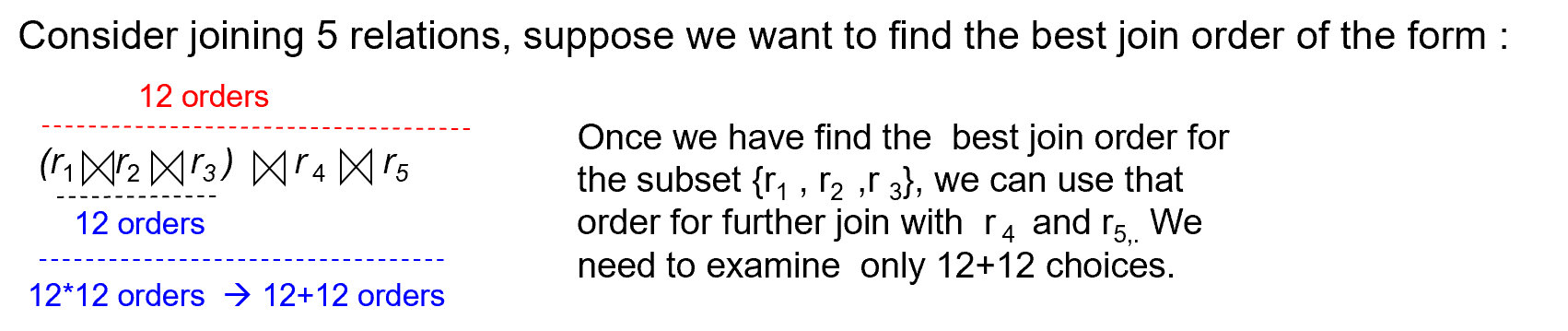
通过动态规划的方式进行连接。比如要连接五个表，确定要先连接前三个表。在前三个表中选择最优的方案（12选1）得到结果表，然后把剩下r4，r5和结果表组合在一起，再选择最优的方案（12选一）进行连接。一共只有24中选择

Using dynamic programming, the least-cost join order for any subset of \(\{r_1, r_2, \ldots r_n\}\) is computed only once and stored for future use.

使用动态规划，任何子集 ${𝑟1,𝑟2,…𝑟𝑛} $的最低成本连接顺序仅计算一次并存储以备将来使用。

Join Order Optimization Algorithm

先分解成两个小的集合 \(S_1, S-S_1\). 递归地细分。

递归到最底层就变为了对单个表的选择方法。

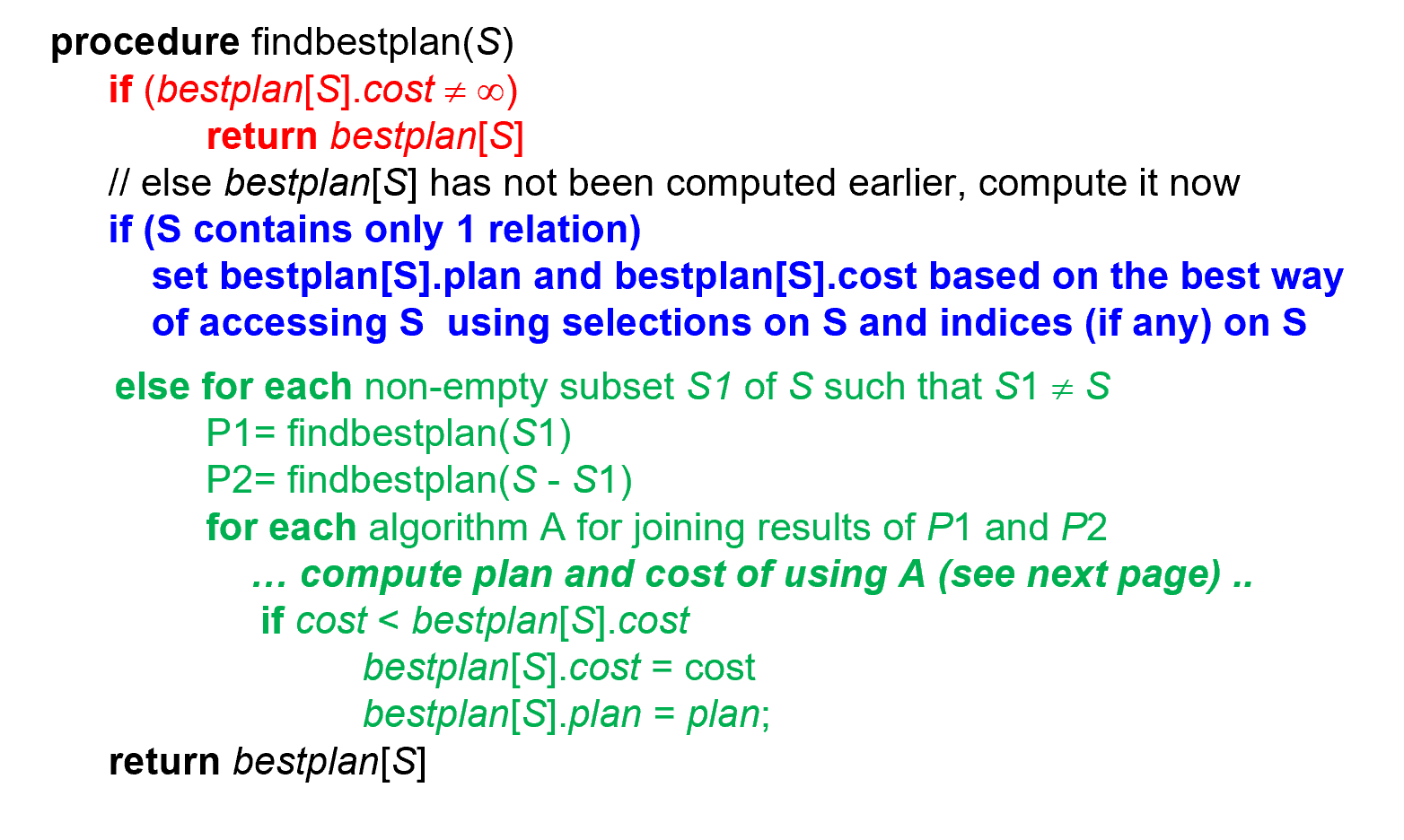
每次将要连接的表分为两个子序列，利用动态规划，所有序列长度小于当前序列的集合最佳排列方式和cost都已知，且保留下来。这样我们就可以不断通过变化两个子序列的长度，计算出当前序列最佳的排列方式和cost

时间复杂度为\(O(3^n)\)，空间复杂度为\(O(2^n)\)

12.4.1.2 Left Deep Join Trees

In left-deep join trees, the right-hand-side input for each join is a relation, not the result of an intermediate join.

在左深连接树中，每个连接的右侧输入是一个关系，而不是中间连接的结果。

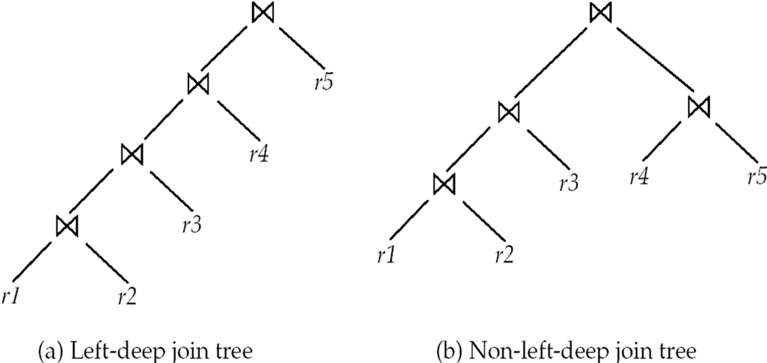
左边可以是中间结果，右边必须是一个关系。

构建左深连接树，对最初始的连接序列S，每次选取最后一个关系，将S分为S-r和r，而不是对于S的任意一个非空子集进行分割。

12.4.1.3 Cost of Optimization

• With dynamic programming
  • time complexity of optimization with bushy trees is \(O(3^n)\).
  • Space complexity is \(O(2^n)\)
• left-deep join tree
  • Time complexity of finding best join order is \(O(n 2^n)\)
  • Space complexity remains at \(O(2^n)\)

12.4.2 Heuristic Optimization

Cost-based optimization is expensive. 可以用启发式优化

Heuristic optimization transforms the query-tree by using a set of rules that typically (but not in all cases) improve execution performance:

启发式优化通过使用一组规则来转换查询树，这些规则通常（但不是在所有情况下）都会提高执行性能：

• Perform selection early (reduces the number of tuples)

  尽早进行选择操作。（减少中间结果元组个数）

• Perform projection early (reduces the number of attributes)

  尽早进行投影操作。（减少中间结果属性个数）

• Perform most restrictive selection and join operations (i.e. with smallest result size) before other similar operations.

  在其他类似操作之前执行限制性最强的选择（select）和连接（join）操作（减少中间结果规模）。

• Perform left-deep join order

  利用左深连接树进行连接。即在为连接操作序列选择最优方案的时候，每次将序列S分为S-r与r，对这两个表选择最优连接方案。(减少时间复杂度)

12.5 Additional Optimization Techniques

12.5.1 Nested Subqueries

优化嵌套查询

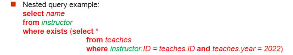
select name 
from instructor 
where exists 
    (select * 
     from teaches
     where instructor.ID = teaches.ID and teaches.year = 2022)

对于每一个教师，把教师的ID在teaches表中进行循环，查看是否有条件满足的记录。

这相当于一个两重循环。外循环是instructor表，内循环是teaches表，效率较低。

Parameters are variables from outer level query that are used in the nested subquery; such variables are called correlation variables（相关变量）

假如说嵌套查询，没有出现在外面的表中的某个属性，例如此处的instructor.ID，那么我们只需先把里面year = 2022的查询好，再与外面的表连接即可

即来自外循环的变量。如果没有相关变量，我们可以先执行内部，然后再执行外部。

优化方法1：嵌套查询改变为连接

select  name
from   instructor, teaches
where instructor.ID = teaches.ID and teaches.year = 2022

把刚刚那个例子改为一个 select 语句，那么一个老师如果开了很多门课就会出现很多个名字。但是加上 distinct 关键词后又无法区分同名情况。

最终我们使用半连接（semijoin）进行优化。半连接的含义是：

\(r\ltimes_\theta s\) Is a subset of r, in which every tuple \(r_i\) matches at least one tuple \(s_i\) in s under the condition \(\theta\).

保留 \(r\) 中能与 \(s\) 相连的元组。

$$ r \ltimes_{\theta} s = \prod_R(r \bowtie _{\theta} s) $$

最终嵌套查询可以写作：

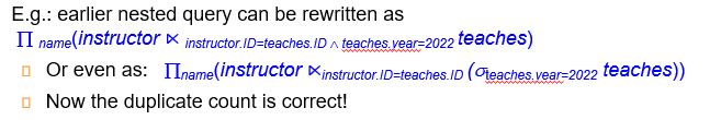
The above relational algebra query is also equivalent to

select name
from instructor
where ID in (select teaches.ID 
                from teaches
                where teaches.year = 2022)

对嵌套查询优化的一般形式：

其中\(P_2^2\)表示与外循环有关的属性

\(P_2^1\)表示只与内循环有关的属性

所以先用\(\sigma_{P_2^1}(s1 \times s2 ...\times s_m)\),先进行选择，然后再用相关变量作为作为半连接的连接条件

The process of replacing a nested query by a query with a join/semijoin (possibly with a temporary relation) is called decorrelation(去除相关)

另一个优化嵌套查询的例子：

Decorrelation of scalar aggregate subqueries can be done using group by/aggregation in some cases

• 先利用teaches_year对teaches表格进行筛选
• 再利用TID进行分组，在每一组中算出教课的数目。
• 半连接时，实际上被半连接的表是一个只有两个属性的表：TID,cnt。
• 利用这个表，对instructor的元组进行筛选，将半连接条件设置为ID = TID& 1 < cnt。因此，instructor表中满足这个条件的ID所在的行元组就会被保留，不满足的行元组会被舍弃。
• 最后，对半连接结果（即选择后的instructor表）进行投影，得到最终的结果。

12.4.2 Materialized Views

A materialized view is a view whose contents are computed and stored.

有些数据库里把 view 实例化了，真正存储在内部的临时表。

create view department_total_salary(dept_name, total_salary)as 
select dept_name, sum(salary) 
from instructor 
group by dept_name

Materializing the above view would be very useful if the total salary by department is required frequently

Saves the effort of finding multiple tuples and adding up their amounts

节省查找多个元组并将其金额相加的精力，使用前提往往是上述视图使用频繁

缺点：但是需要时刻保持这个视图和原表一致。

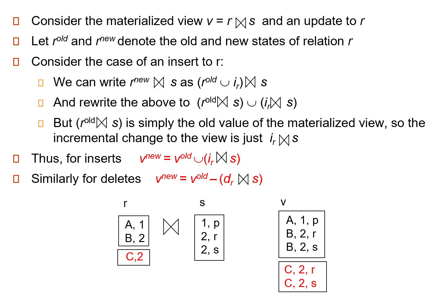
use incremental view maintenance(增量视图维护) ：Changes to database relations are used to compute changes to the materialized view, which is then updated

对数据库关系的更改用于计算对物化视图的更改，然后更新物化视图

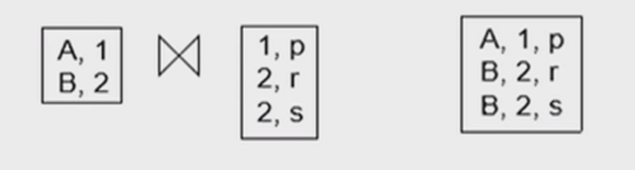
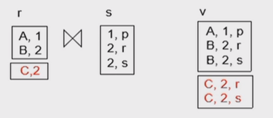
The changes (inserts and deletes) to a relation or expressions are referred to as its differential(差分)： Set of tuples inserted to and deleted from r are denoted \(i_r\) and \(d_r\)

例如，最初，两个表连接结果如下：

现在，表格r插入了一条新的记录：

那么，需要将新增的这条记录和s表做连接，并将连接的结果加入到物化视图中，以维护视图信息的正确性。

• join: \(V^{new}=V^{old}\cup (i_r\bowtie s), V^{new} = V^{old}-(d_r\bowtie s)\)

  

• select: \(V^{new}=V^{old}\cup \sigma_\theta(i_r), V^{new} = V^{old}-\sigma_\theta(d_r)\)

  假如不是连接操作，这个物化视图是由另一个表r的选择操作得出的。那么假如表r插入了一条新元组，为了维护物化视图，只要把插进去的那个元组利用相同的选择条件进行选择，如果选择上了，就把它并到物化视图中。

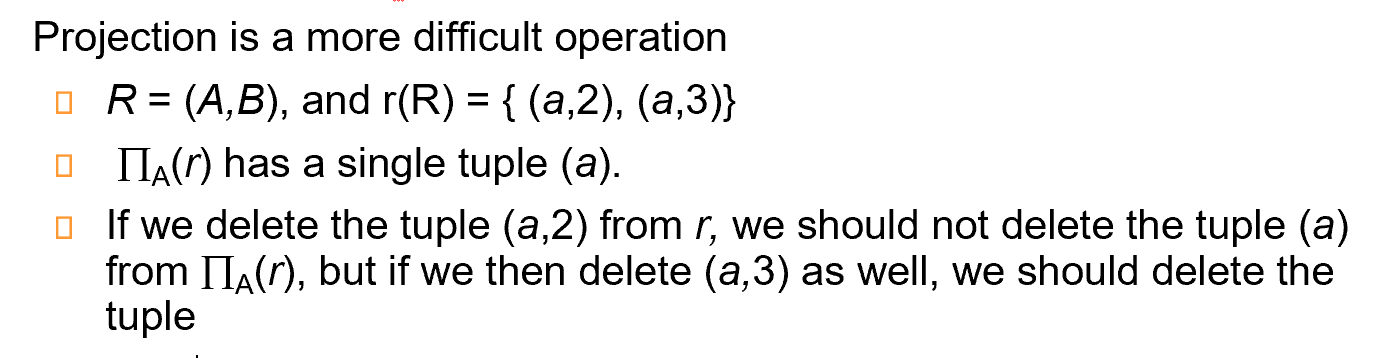
• projection:

  For each tuple in a projection \(\Pi_A(r)\), we will keep a count of how many times it was derived.

  • On insert of a tuple to r, if the resultant tuple is already in \(\Pi_A(r)\) we increment its count, else we add a new tuple with count = 1

  • On delete of a tuple from r, we decrement the count of the corresponding tuple in \(\Pi_A(r)\)

    • if the count becomes 0, we delete the tuple from \(\Pi_A(r)\)
    

• count \(v= _Ag_{count(B)}\)

  • insert: For each tuple r in \(i_r\), if the corresponding group is already present in v, weincrement its count, else we add a new tuple with count = 1

  • delete: for each tuple t in \(i_r\).we look for the group t.A in v, and subtract 1 from the count for the group.

  If the count becomes 0, we delete from v the tuple for the group t.A

  假如物化视图是由对A属性对表r进行分组，然后进行count计算得到的，那么假设表r新插入了一条元组，假设这个元组的分组属性的值在分好组的分组属性值的集合中，那么就把对应物化视图的这个count值加1。假设这个元组的分组属性的值不在分好组的分组属性值中，那么就在物化视图中插入新的一行，包括这个元组的分组属性值，对应的count置为1。

• sum \(v= _Ag_{sum(B)}\)

  与count类似。当插入一条新的元组时，我们需要add这个元组中属性A的value

  由于存在value=0的情况，我们还需要记录count来检查groups中是否存在tuple。而不能简单依靠sum=0进行判断

  To handle the case of avg, we maintain the sum and count aggregate values separately, and divide at the end。对于平均数的维护，分别维护sum和count，最终相处进行计算

• min, max：\(v = _Ag_{min(B)}(r)\)

  1. 对于插入的处理较为简单，比较一下现有的min和max即可
  2. 维护删除时的最小值和最大值的聚合值可能会更昂贵。 我们必须查看同一组中的其他元组以找到新的最小值(可能会把最小值或者最大值删除，这是需要重新寻找)

• set intersection: \(v = r \cap s\)

  1. 当一个元组插入到 r 中时，我们检查它是否存在于 s 中，如果存在，我们将其添加到 v 中。
  2. 如果从 r 中删除该元组，则我们将其从交集中删除（如果存在）。

怎么利用这些 view?

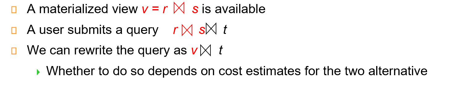
• Rewriting queries to use materialized views:

  

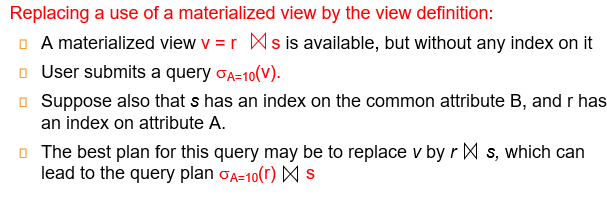
• Replacing a use of a materialized view by the view definition

  

Materialized View Selection

有哪些查询？各种查询的比例？